Transcription
Proc. of IEEE Intl. Conf. on Multisensor Fusion and Integration for Intelligent Systems (MFI), 2017, Daegu, Korea. DOI: 10.1109/MFI.2017.8170347c 2017 IEEE. Personal use of this material is permitted. Permission from IEEE must be obtained for all other uses, in any current or future media, including reprinting/republishing this material for advertising or promotional purposes, creatingnew collective works, for resale or redistribution to servers or lists, or reuse of any copyrighted component of this work in other works.Dynamic Covariance Estimation – A Parameter Free Approach toRobust Sensor FusionTim Pfeifer, Sven Lange and Peter ProtzelDept. of Electrical Engineering and Information TechnologyTU Chemnitz, GermanyEmail: {firstname.lastname}@etit.tu-chemnitz.deI. I NTRODUCTIONThe probabilistic fusion of different kinds of sensor datais an extensively explored field of research. In robotics,the special case of simultaneous localization and mapping(SLAM) was solved by different techniques like Kalmanor particle filter, but the de facto standard are optimizationbased algorithms. These algorithms reformulate the sensorfusion problem into a non-linear least squares optimization.While the least squares problem contains the probabilisticrelations between sensor data and the states of a system, anoptimization back-end is used to find the most likely systemstate. GTSAM [1] and Ceres [2] are just two examples forthe most common optimization back-ends in recent roboticapplications.Standard least squares optimization is based on the ideaof Gaussian distributed measurement noise with a knownvariance. However, many real world applications violate thisessential assumption. Our motivation in this context are GNSSbased navigation systems like GPS as well as local wirelesslocalization systems. They suffer form multipath and nonline-of-sight (NLOS) effects and cause heavy tailed or evenmulti-modal error distributions. Although they are boundedin range, their shape is non-Gaussian and changes with theproperties of the environment like the height of buildingsThe project is funded by the ”Bundesministerium für Wirtschaft undEnergie” (German Federal Ministry for Economic Affairs and Energy).2.5Ground TruthGaussianDCE21.5Y [m]Abstract— In robotics, non-linear least squares estimation isa common technique for simultaneous localization and mapping.One of the remaining challenges are measurement outliers leading to inconsistency or even divergence within the optimizationprocess. Recently, several approaches for robust state estimationdealing with outliers inside the optimization back-end werepresented, but all of them include at least one arbitrary tuningparameter that has to be set manually for each new application.Under changing environmental conditions, this can lead to poorconvergence properties and erroneous estimates. To overcomethis insufficiency, we propose a novel robust algorithm basedon a parameter free probabilistic foundation called DynamicCovariance Estimation. We derive our algorithm directly fromthe probabilistic formulation of a Gaussian maximum likelihoodestimator. Through including its covariance in the optimizationproblem, we empower the optimizer to approximate these to thesensor’s real properties. Finally, we prove the robustness of ourapproach on a real world wireless localization application wheretwo similar state-of-the-art algorithms fail without extensiveparameter tuning.10.5000.511.522.5X [m]Fig. 1. The figure shows the estimated trajectory of our robot, equippedwith a wireless localization system. Non-Gaussian outliers cause a distortionof the non-robust estimate. The proposed Dynamic Covariance Estimation(DCE) algorithm offers robustness against erroneous measurements withoutmanual parameter tuning.or the position of reflecting objects. Other examples areoptical sensors which can be influenced by bad weather orchallenging lighting conditions and wheel odometry whichcan be affected by slipping on difficult grounds. These errorscan not be estimated online without additional sensor dataand possibly distort the estimated system state significantly.In the past, several algorithms were proposed to improvethe back-end robustness for SLAM applications [3]–[8]. Themajority of them can be divided in two groups, one triesto model a non-Gaussian error distribution while the othertries to weight down measurements that don’t fit to a Gaussdistribution.In [9] we compared representatives from both groups.While the down weighting is advantageous for small outlierratios, the probabilistic modeling approach seems to be amore general solution. The downside of all algorithms is therequirement of parametrization, since all of them introduce
at least one additional parameter compared to standard leastsquares. Corresponding to the concept of the algorithm, theseparameters describe a probabilistic distribution or can bearbitrary. While a distribution’s parameter can be estimatedby statistical methods, the arbitrary parameters have to betuned manually. Likewise, both can be extremely difficult ifthe error distribution vary over time.In this paper, we want to introduce an approach that combines the robust down-weighting of Switchable Constraints(SC) with a probabilistic consistent design that is able toparametrize itself. Hence, we propose the novel DynamicCovariance Estimation (DCE) algorithm that does not requireany new parameter compared to standard least squares. Weachieve this by including the variance of the sensor in theoptimization process, as an additional state variable. Similarto Dynamic Covariance Scaling (DCS), we also provide ananalytically optimized closed form alternative which can beexpressed as an m-estimator. Finally, we validate both variantswith a real world wireless localization system (see Figure 1)in comparison to SC and DCS.II. R ELATED W ORKWith the rising popularity of SLAM in the past decade, abroad variety of methods were proposed to achieve robustnessagainst wrong data association and outliers. While SLAM canbe viewed as special case of sensor data fusion, the majorityof these techniques can be applied to general sensor fusionproblems, as we showed in [9] or [10]. The common basisof these algorithms is (1) which maximizes the probabilityof the state variables X for a given set of measurements Z.YX argmaxP (xi zi )(1)XiThe transformation of this maximum likelihood estimatorfor X to a non-linear least squares problem (2)1 is possibleunder assuming a Gaussian distribution for P (xi zi ). Forsimplicity, we consider the one dimensional case, but thealgorithm applies also to multidimensional problems.XX argmink e(xi , zi ) k2Σ(2) {z }XieiDue to the vulnerability of least squares against outliers,the existing robust approaches modify this equation to limitor prevent the outliers influence. Max Mixture [6], [11] andgeneralized iSAM [7] wrap the error function ei with aprobabilistic model superior to a uni-modal Gaussian. Hence,it is possible to approximate an arbitrary error distributionfor a wide variability of non-Gaussian measurement noiseto obtain more realistic estimation results. While these classof algorithms can achieve a high level of robustness, forsensors with unknown or time-dependent distributions, theyare difficult to parametrize.The other class of algorithms is introducing an additionalweight wi to scale each error independently2 .X argminX·k2Σis the squared mahalanobis distance with covariance Σ.valid notation would be ψ kei k2Σ .2 Anotherkwi · ei k2Σ(3)iThese weights can be determined by the optimizer itselfin case of Switchable Constraints (SC) [8], [12], [13] orcalculated as function of ei for Dynamic Covariance Scaling(DCS) [4], [14], [15] and other m-estimators.A. Switchable ConstraintsSC introduced a novelty for robust lest squares, a weight(or switch) s that is directly included in the optimizationprocess. To prevent the trivial solution si 0 i a priorconstraint eSP is added for each switch, which leads to (4).Additionally, a limitation of si between 0 and 1 is required. XX X , S argmin ksi · ei k2Σ k 1 si k2Ξi (4) {z }X,SiieSPiA critical point of SC is the introduction of the newparameter Ξ as covariance of the switch prior eSPi . This tuningconstant adjusts the trade-off between robustness againstoutliers and the tendency to weight valid measurements down.Due to the missing probabilistic relation between Ξ and thedistribution of the sensor, this essential value is difficult todetermine and has to be fine-tuned manually. Nevertheless,there seems to be a certain range of valid values for typicalSLAM datasets [8], but no guarantee can be given that thisalso applies to general sensor fusion problems. In fact, insection VII, we show counterexamples.B. Dynamic Covariance ScalingProposed as improvement of SC, the DCS algorithm appliesan analytical optimization to transform (4) to an m-estimatorsimilar to (3) while calculating each weight with (5). 2Φwith Φ Ξ 1(5)si min 1,Φ kei k2ΣiThrough the closed form, an instantaneous calculation of siprovides a faster convergence while achieving the same levelof robustness compared to original SC. However, it still keepsthe arbitrary tuning variable and all the disadvantages that goalong with manual parameter tuning. In addition, our previouswork [9] showed some potential convergence problems insensor fusion applications.C. Self-tuning M-EstimatorsA parameter free solution for some cases is presented inthe work of Agamennoni et al. [3], where a class of selftuning m-estimators is proposed. With the use of ellipticaldistributions, they are able to include the parameter φ of anm-estimator ψ(·, φ) in the optimization problem. To keepthe log-likelihood and therefore the least squares problempositive, they add a regularization term ln c (ψ)."1kXn 1XX , φ argmin n · ln c (ψ) ψ kei k2Σ2 i 1X,φ #(6)
For many applications this approach proves to be valid. Insome cases however, using the single parameter φ – insteadof the set of weights si S of Switchable Constraints –may be insufficient. Furthermore, the adaptation of φ to atime-variable distribution is ad hoc not possible. Anotherlimitation is the selection of m-estimators. DCS and otherfast descending m-estimators have no corresponding ellipticaldistributions, so the self tuning can not be applied.A common problem of many m-estimators in least squaresproblems is the bad convergence behaviour in case ofinaccurate or incorrect initialization. Papers like [16], [17]address this issue but whether these techniques can be appliedto DCS or the self-tuning m-estimators is unclear.In the following section, we introduce a novel formulationof a robust least squares algorithm that is closely related toSC but parameter free and based on the Gauss distributionitself.III. DYNAMIC C OVARIANCE E STIMATIONWhile Switchable Constraints adds a scaling factor to theerror function, our approach scales the variance (or its root, thestandard deviation) of the assumed error distribution directly.Since the standard deviation also scales the error, this appearsidentical at first glance, but it comes with different side effectson the estimation problem. To get a better understanding, wehave to look at the missing steps between (1) and (2).The transformation from a maximum likelihood estimatorto a non-linear least squares problem is done by applying thenatural logarithm which results in (7).XX argmin ln (P (xi zi ))(7)Xi e2· exp i 2(8)2σ2πσ 2With the probability density function of a zero-meanGaussian (8), the log-likelihood for one measurement can bedescribed as: 1 ln(P (xi zi )) ln2πσ 2 kei k2Σ(9) {z} 2P (xi zi ) 1const.In standard least squares, the constant first part getsneglected. If we add the standard deviation to the estimationprocess on the other hand, this part becomes variable andhas to be included. With this natural regularization term, atrivial solution like σ can be prohibited.To apply this to measurements with a non-constant errordistribution, we replace the constant σ by a set of timedependent variances σi σ. This leads to the new problemformulation in (10) and (11).YX , σ argmaxP (xi , σi zi )(10)X,σ ln(P (xi , σi zi )) ln i q2πσi2{zvariable }1 kei k2Σi2(11)To keep this proposed equation valid for least squaresoptimization, we have to guarantee ln(P (xi , σi zi )) 0,which is not possible for arbitrary σi . Therefore, we set alower bound σmin and shift p(11) by a corresponding constant2regularization term ln2πσmin, similar to Rosen etal. in [7] or the self tuning m-estimators mentioned in II-C.Through reformulation of (12) and step (13), we get our finalDynamic Covariance Estimation formulation (14). Equivalentto SC, DCE can be considered as two separated error functionswhere ln kσi k2Σmin is a non-linear prior. q q1222πσi ln2πσmin kei k2Σi ln(P ) ln2(12) σi1 ln(P ) ln kei k2Σi(13)σmin2 ln(P ) 11ln kσi k2Σmin kei k2Σi22(14)2is the pre-defined covariance of our physicalΣmin σminsensor under normal conditions and can be determinedexperimentally or read from the datasheet. It is not a new freeparameter since all other algorithms including the non-robustleast squares also require this fundamental parameter. Inconsequence, we allow the optimizer to reduce the weight oferroneous measurements while preventing an overfitting of theexact ones. An advantage over m-estimator based approachesis the convex surface of the error term 12 kei k2Σi which allows awell-behaved convergence. However, in common with SC, wehave the computational burden of additional state variables.IV. C LOSED F ORM DCESimilar to the transformation between SC and DCS, throughanalytical optimization of DCE a closed form m-estimatorcan be provided. The optimization can be described with(15), where the error value ei is treated as constant.σi argmaxσi11ln kσi k2Σmin kei k2Σi22(15)The maximum of this log-likelihood exists for σi ei .Under the condition σi σmin , two cases have to bedifferentiated:(σmin if ei σmin (16)σi ei if ei σminThrough substituting σi in (14) with (16) the resultingequation describes the closed form m-estimator of DCE(cDCE).(122 kei kΣi122 ln kei kΣminif ei σminif ei σmin(17)With σmin , (17) requires the same probabilistic parameteras DCE. However, this parameter is quite simple to determine,as mentioned before. ln(P (xi zi )) 12
While the resulting log-likelihood of DCE and cDCE isidentical, there is no guarantee for an identical convergencebehaviour. Since DCE (as well as SC) treats the varianceand the resulting error as separate dimensions during theoptimization, it can converge differently compared to cDCE.Therefore, we expect a better convergence of DCE similar toSC (compared to DCS) in our former work [9].When applying cDCE it is important to remember the tradeoff between robustness and convergence that all m-estimatorsshare. Compared to DCS, we pushed this compromise closerto a better convergence but keep a decent level of robustnessas Figure 2 shows.GaussianDCScDCEWeighted Squared Errorq22x,yM odkxx,y zirngM od xi k ci(18)Σrng6B. Odometry Model543210-15Through Time-of-Flight measurement, the UWB modulesprovide an absolute distance between itself xx,yM od and theposition of our robot xx,y.InadditiontoaGaussiannoiseiand the NLOS errors, each range measurement zirng containsoda certain offset cMcaused by the physical properties of theiantenna. This antenna offset depends on the orientation anddistance between transmitter and receiver and is estimatedfor each module independently. With (18) the correspondingerror function is provided.erng i87A. Range Error Model-10-5051015ErrorFig. 2. Each error term adds a weighted and squared error to the optimizationprocess. Robust weight-functions limit the influence of these terms. ThecDCE m-estimator provide less robustness against extreme outliers, but betterconvergence properties than DCS.The state transition between poses as well as the initialization of new ones is based on a motion model of a differentialdrive robot. By using both wheels’ velocity measurementas input, the error function is given as eodoi . Since a twowheeled differential drive robot is non-holonomic, the velocityperpendicular to the driving direction also has to be consideredto formulate a well-posed estimation problem. We assumethese to have a zero mean, which results in a measurement vector ziodo [ vl , vr , vy 0 ] that contains one additionalentry along with the wheel velocities. 1eodo T · (xx,y,φ xx,y,φ ziodoiii 1 ) tV. L OCALIZATION AS FACTOR G RAPHA basic class of sensor fusion problems is the positionestimation based on multiple data sources, generally calledlocalization. Our Evaluation is focused on a specific case,where relative wheel odometry is combined with an set ofabsolute range measurements to fixed points. To examine thestructure of this estimation problem, we can describe it asa factor graph as shown in Figure 3. This graphical modelshows the probabilistic connections (small dots) betweenthe state variables (big circles). In the following section weexplain these connections, also called error functions, thatdefine our estimation problem.x42Σodo(19)The formulation of (19) in the measurement space, requiresa transformation from two consecutive global poses to a setof differential drive velocities with the matrix T . Therefore,(20) contains a rotation from a global to a local coordinateframe combined with the inverse kinematic of a differentialdrive robot. xφi denotes the rotational component of the 2Dpose and 2 · dw the distance between both wheels. 1T 10 001 cos xφisin xφi dwφdw · sin xicos xφi000{z} {zdifferential kinematicrotation 00 (20)1}C. Constant Offset ModelFig. 3. Factor graph of the least squares problem. Big circles representstate variables while small circles are the probabilistic connections betweenthese variables. The dotted switch or standard deviation variable is onlyadded for SC or DCE. Note that the framed range and offset factors arepresent 4 times.f setThe module specific offset eofis caused by the influience of the antenna on the electromagnetic wave propagation.Not only the physical characteristics but also the alignment ofthe antennas affect this value. Therefore, a continuous distanceand orientation variation caused by the robot’s movement,requires also a continuous offset estimation. To ensure theodconsistency of cMover time we use a simple constant valueimodel (21).f seteof i ododcM cM· t 1ii 12Σof f set(21)
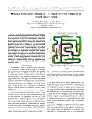
0.060.060.040.040.020.020-0.200.20.40-0.20.6Range Error [m]0.060.060.040.040.020.020-0.200.20.40.6Range Error [m]Fig. 4. Our robotic system inside the labyrinth, seen from the trackingsystem. One UWB module is placed in each corner and one on top of therobot. The white paper sheets contain two layer of aluminium foil to enforceNLOS measurements.VI. E XPERIMENTTo explore the different robustness and convergence properties, we decided to evaluate our proposed DCE/cDCEalgorithm along with SC and DCS on a real world dataset.Based on our experience with a synthetic benchmark in[9], we designed an equivalent setup with one of our smalleducational robots [18] that navigates through a labyrinth.Due to the flat surface, we reduced this to a two-dimensionallocalization problem. As ground truth for evaluation, anoptical mono-camera tracking system as introduced in [19]is used. We adapted this system to the 2D case and achievea centimetre-level accuracy, which is sufficient for ourcomparison. Our final dataset contains about 15 minutesof continuous driving.A. Wireless Localization DatasetFor long term consistent localization, the wheel odometry iscomplemented by a set of five wireless ranging sensors. Oneon top of the robot and one in each corner of the labyrinth asseen in Figure 4. Once each time step, the robot measures thedistance to one of the static modules. These ultra-widebandsensors [20] are ideal to compare robust algorithms, since theysuffer from non-Gaussian error distributions. While they areinherent robust against multipath effects, they cannot measurea correct distance if the direct line-of-sight is blocked byan obstacle. In these NLOS cases, the measured distance issignificantly longer than the real one. The resulting heavytailed distribution is challenging for non-robust optimization.So the corresponding error function is robustified by our setof algorithms. Obstacles could be walls, furniture or humansfor indoor applications or entire buildings in satellite basedlocalization applications. We enforce a decent amount ofNLOS measurements with artificial walls, made of aluminiumfoil.00.20.40.6Range Error [m]0-0.200.20.40.6Range Error [m]Fig. 5. These histograms show the error distributions of the wireless distancemeasurements to the 4 fixed modules. Due to the geometric differences inthe labyrinth they can differ. All distributions are asymmetric and contain adifferent amount of outliers.B. ParametrizationAll factors included in Figure 3 require a covariancefor each dimension of the particular error function. Theseare summarized in Table I. A correct parametrization ofthese covariances is mandatory for a meaningful comparison.Hence, we estimated these values very carefully in separateexperiments. By using the visual ground truth, we estimatedthe odometry’s standard deviation over several minutes ofdriving. The standard deviation of our wireless distancemeasurements was determined outdoors in a flat environment.Under this free space conditions, we were able to measure thesensors noise. A separate test-drive under LOS conditions thecompleted the characterization of the UWB sensors with theconstant offset model’s covariance. The covariance of the usedpriors is the only one that we set manually. It represents theknowledge about the robot’s start state which is limited sincewe only know that the robot is somewhere in the labyrinth.TABLE IC OVARIANCES OF THE ESTIMATION PROBLEMmodelerror functioncovariancedistance measurementerngiwheel odometryeodoiconstant offset modelf seteofiΣrng [0.025 m]2 20.03 m s 1 1 Σodo diag 0.03 m s 0.03 m s 1 2Σof f set 1 mm s 1antenna offset priorepriorof f setpose prioreposeprior2Σpriorof f set [0.1 m] 210 mpose Σprior diag 10 m 2π rad
We implemented our least squares problem with the Ceressolver [2] as optimization back-end. While the growingestimation problem would violate any real time condition, weapply a sliding window approach to exclude old state variablesfrom optimization. The length of the time window balancesthe trade-off between computation time and estimation quality.We choose a length of 10 s to keep the required optimizationtime bounded without losing noteworthy precision.All of these algorithms are able to suppress the influence ofoutliers to the resulting estimate. Especially the maximumtrajectory error is reduced by almost 50% as shown in Figure 7.However, as summarized in Table II, SC as well as DCS failto converge on this problem with their tuning parameterset to 1. Therefore, both algorithms cannot improve theestimation result over the bare odometry initialization withthe recommended parametrization.VII. R ESULTSTABLE IIR ESULTS OF THE FINAL RUNA. Parameter Tuning of SC and DCSThe performance of SC and DCS depends strongly onthe chosen tuning parameter. To show this dependency, weperformed several runs of both algorithms with a different parametrization. Figure 6 plots the resulting absolutetrajectory error (ATE) [21] for parameter values betweenξ 0.001 and 1.6.AlgorithmOdometry InitialGaussianDCEcDCESC (Ξ 1.0)SC (Ξ 0.2)DCS (Φ 1.0)DCS (Φ 10)7SC meanSC maxDCS meanDCS max6ATEPOS [m]540.330.252Time 8014.97430.16934.30510.1806ATEPOS 1ξ0.05Fig. 6. Our parameter evaluation of SC and DCS shows the absolutetrajectory error for different parameter values ξ. SC applies Ξ ξ whileDCS uses the inverse Φ ξ 1 . Only a small range between 0.1 and 0.25offers an optimal performance.According to our results, DCS and SC converge only forvalues of ξ below 0.25. Values smaller than 0.1 don’t breakthe optimization process but lead to a performance identicalto the non-robust optimization. In the final comparison, weused the best parametrization for both algorithms. Hence,SC uses a Ξ of 0.2 and DCS a Φ of 10. Compared tothe results of DCS in [4] and [14], we got a significantlysmaller range of valid values. In case of SC there is an evenmore distinct difference to [22], where a range of 0.3 to1.5 is recommended. These tests were performed on SLAMdatasets with synthetic error distributions, unclear covariancesand different optimization back-ends, which could explainsome of the discrepancies. Furthermore, our sliding windowapproach can be more challenging than the batch optimizationin previous publications.B. Final EvaluationSince the performance of SC and DCS depends on thetuning parameters, we included two parameter sets to ourcomparison. We run both with their default parameter of 1.0and with the prior tuned parameters, which lead to differentresults. Our proposed DCE/cDCE algorithms achieved thesame results as the manually tuned SC and DCS versions.0GaussianDCEcDCEFig. 7. Absolute Trajectory error of the estimated positions. DCE/cDCEas well as tuned SC/DCS performed well, but standard SC/DCS failed toconverge.The accumulated runtime of the sliding window filter givenin Table II was measured on an Intel i7-4770 system. Tomention is the advantage of the closed form algorithms (DCSand cDCE), both require less computational time then theirrespectively alternatives with additional state variables. Also,DCE and cDCE require more time to converge to a finalsolution but compared to the dataset length of 930 seconds,all algorithms are sufficiently fast.VIII. C ONCLUSIONWe introduced a novel robust estimation algorithm whichwas designed with a probabilistic foundation and withoutthe introduction of an arbitrary tuning constant. The basicidea is to include the covariance of the sensor itself to theoptimization process. Furthermore, we derived a closed formalternative to our Dynamic Covariance Estimation algorithm,providing comparable robustness with reduced computationalcost. We compared both variants to the similar SwitchableConstraints and Dynamic Covariance Scaling algorithm on areal world wireless localization dataset. So we were able toshow the advantage of our parameter free algorithms since SC
and DCS perform only equivalent with extensive parametertuning in advance.In our future work, we will extend this comparison todifferent datasets to generalize our observations from thisspecific setting. Furthermore, an evaluation of the theoreticalproperties of the DCE algorithm will be useful to expose therelationship between the estimated and the real covariance.An analysis of possible probabilistic connections between theindividual covariance variables could also be very interestingin this context.R EFERENCES[1] F. Dellaert and Others, “GTSAM,” http://research.cc.gatech.edu/borg/gtsam.[2] S. Agarwal, K. Mierle, and Others, “Ceres Solver,” http://ceres-solver.org.[3] G. Agamennoni, P. Furgale, and R. Siegwart, “Self-tuning m-estimators,”in Proc. of Intl. Conf. on Robotics and Automation (ICRA), 2015.[4] P. Agarwal, G. D. Tipaldi, L. Spinello, C. Stachniss, and W. Burgard,“Robust map optimization using dynamic covariance scaling,” in Proc.of Intl. Conf. on Robotics and Automation (ICRA), 2013.[5] Y. Latif, C. Cadena, and J. Neira, “Robust loop closing over time forpose graph SLAM,” Intl. Journal of Robotics Research, 2013.[6] E. Olson and P. Agarwal, “Inference on networks of mixtures for robustrobot mapping,” Intl. Journal of Robotics Research, 2013.[7] D. M. Rosen, M. Kaess, and J. J. Leonard, “Robust incremental onlineinference over sparse factor graphs: Beyond the Gaussian case,” inProc. of Intl. Conf. on Robotics and Automation (ICRA), 2013.[8] N. Sünderhauf and P. Protzel, “Switchable constraints for robust posegraph slam,” in Proc. of Intl. Conf. on Intelligent Robots and Systems(IROS), 2012.[9] T. Pfeifer, P. Weissig, S. Lange, and P. Protzel, “Robust factor graphoptimization – a comparison for sensor fusion applications,” in Proc. ofIntl. Conf. on Emerging Technologies and Factory Automation (ETFA),2016.[10] S. Lange, N. Sünderhauf, and P. Protzel, “Incremental smoothing vs.filtering for sensor fusion on an indoor UAV,” in Proc. of Intl. Conf.on Robotics and Automation (ICRA), 2013.[11] R. Morton and E. Olson, “Robust sensor characterization via maxmixture models: GPS sensors,” in Proc. of Intl. Conf. on IntelligentRobots and Systems (IROS), 2013.[12] N. Sünderhauf, M. Obst, S. Lange, G. Wanielik, and P. Protzel,“Switchable constraints and incremental smoothing for online mitigationof non-line-of-sight and multipath effects,” in Proc. of IntelligentVehicles Symposium (IV), 2013.[13] N. Sünderhauf and P. Protzel, “Switchable constraints vs. max-mixturemodels vs. rrr – a comparison of three approaches to robust pose graphSLAM,” in Proc. of Intl. Conf. on Robotics and Automation (ICRA),2013.[14] P. Agarwal, G. Grisetti, G. Diego Tipaldi, L. Spinello, W. Burgard, andC. Stachniss, “Experimental analysis of dynamic covariance scalingfor robust map optimization under bad initial estimates,” in Proc. ofIntl. Conf. on Robotics and Automation (ICRA), 2014.[15] P. Agarwal, “Robust graph-based localization and mapping,” Ph.D.dissertation, University of Freiburg, 2015.[16] D. M. Rosen, C. DuHadway, and J. J. Leonard, “A convex relaxationfor approximate global optimization in simultaneous localization andmapping,” in Proc. of Intl. Conf. on Robotics and Automation (ICRA),2015.[17] J. Wang and E. Olson, “Robust pose graph optimization using stochasticgradient descent,” in Proc. of Intl. Conf. on Robotics an
along with manual parameter tuning. In addition, our previous work [9] showed some potential convergence problems in sensor fusion applications. C. Self-tuning M-Estimators A parameter free solution for some cases is presented in the work of Agamennoni et al. [3], where a class of self tuning m-estimators is proposed. With the use of elliptical