Transcription
doi.org/10.26434/chemrxiv.13483335.v1Machine Learning-Based Model Selection and Parameter Estimationfrom Kinetic Data of Complex First-Order Reaction SystemsLászló Zimányi, Áron Sipos, Ferenc Sarlós, Rita Nagypál, Géza GromaSubmitted date: 23/12/2020 Posted date: 24/12/2020Licence: CC BY-NC-ND 4.0Citation information: Zimányi, László; Sipos, Áron; Sarlós, Ferenc; Nagypál, Rita; Groma, Géza (2020):Machine Learning-Based Model Selection and Parameter Estimation from Kinetic Data of ComplexFirst-Order Reaction Systems. ChemRxiv. Preprint. ng with a system of first-order reactions is a recurrent problem in chemometrics, especially in theanalysis of data obtained by spectroscopic methods. Here we argue that global multiexponential fitting, the stillcommon way to solve this kind of problems has serious weaknesses, in contrast to the available contemporarymethods of sparse modeling. Combining the advantages of group-lasso and elastic net – the statisticalmethods proven to be very powerful in other areas – we obtained an optimization problem tunable to result infrom very sparse to very dense distribution over a large pre-defined grid of time constants, fitting bothsimulated and experimental multiwavelength spectroscopic data with very high performance. Moreover, it wasfound that the optimal values of the tuning hyperparameters can be selected by a machine-learning algorithmbased on a Bayesian optimization procedure, utilizing a widely used and a novel version of cross-validation.The applied algorithm recovered very exactly the true sparse kinetic parameters of an extremely complexsimulated model of the bacteriorhodopsin photocycle, as well as the wide peak of hypothetical distributedkinetics in the presence of different levels of noise. It also performed well in the analysis of the ultrafastexperimental fluorescence kinetics data detected on the coenzyme FAD in a very wide logarithmic timewindow.File list (2)FOkin ms.pdf (1.92 MiB)view on ChemRxivdownload fileFOkin si.pdf (0.91 MiB)view on ChemRxivdownload file
Machine learning-based model selection andparameter estimation from kinetic data of complexfirst-order reaction systemsLászló Zimányi1, Áron Sipos1, Ferenc Sarlós1, Rita Nagypál1,2 and Géza I. Groma1*1Institute of Biophysics, Biological Research Centre, H-6701, Szeged, Hungary2Doctoral School of Physics, University of Szeged, H-6720, Szeged, HungaryKeywords: chemometrics, exponential fitting, sparse modeling, lasso, elastic net, crossvalidation, Bayesian optimization, bacteriorhodopsin photocycle, FAD fluorescence kinetics1
ABSTRACTDealing with a system of first-order reactions is a recurrent problem in chemometrics, especiallyin the analysis of data obtained by spectroscopic methods. Here we argue that globalmultiexponential fitting, the still common way to solve this kind of problems has seriousweaknesses, in contrast to the available contemporary methods of sparse modeling. Combining theadvantages of group-lasso and elastic net – the statistical methods proven to be very powerful inother areas – we obtained an optimization problem tunable to result in from very sparse to verydense distribution over a large pre-defined grid of time constants, fitting both simulated andexperimental multiwavelength spectroscopic data with very high performance. Moreover, it wasfound that the optimal values of the tuning hyperparameters can be selected by a machine-learningalgorithm based on a Bayesian optimization procedure, utilizing a widely used and a novel versionof cross-validation. The applied algorithm recovered very exactly the true sparse kineticparameters of an extremely complex simulated model of the bacteriorhodopsin photocycle, as wellas the wide peak of hypothetical distributed kinetics in the presence of different levels of noise. Italso performed well in the analysis of the ultrafast experimental fluorescence kinetics data detectedon the coenzyme FAD in a very wide logarithmic time window.INTRODUCTIONFrom classical flash photolysis1-8 to the recent methods of ultrafast time-resolved spectroscopy,914light-induced kinetic studies – especially those carried out on macromolecules – face thechallenge of analyzing a complex scheme of reactions. One reason for such a complexity is relatedto the lengthy cascade of the reactions initiated by photoexcitation. A typical example of that isthe sequence of photointermediates of retinal proteins, including the very complicated scheme of2
bacteriorhodopsin (bR)15 photocycle. Another reason of complexity lies in the heterogeneity of theconformational states and/or the microenvironment of a chromophore studied by time-resolvedfluorescence9, 11 or transient absorption.14 Regardless of the degree of complexity, in most of theabove problems it can be supposed that the individual steps of the reaction scheme can be wellapproximated by first-order kinetics. In such a case the problems can be handled by the standardmethods for solving a system of linear homogeneous differential equations of first order.16-18Briefly, a given scheme of n reaction components can be characterized by an n n microscopicrate matrix K , the non-diagonal Ki , j elements of which represent the rate constant of the reactionfrom component j to component i , and K i ,i is the negative sums of the outward rates fromcomponent i . The corresponding macroscopic rate constant and decay-associated spectra (DAS)or difference spectra (DADS)18 – characterizing the experimentally observable kinetic data – canbe calculated by solving the eigenvalue problem of K , with satisfying the initial conditions. Dueto the existence of constraints among the elements of the matrix, its eigenvalues are always real.17If the eigenvalues are also non-degenerate, as generally supposed in routine analyses, the solutionof the above system of differential equations can be expressed as a sum of exponential terms.From the viewpoint of the experimentalist, the problem to solve is just the reverse of the schemeoutlined above. In most cases the observed data do not hold direct information on the timedependent concentration of the reaction components. Instead, the data typically originate from akind of spectroscopic experiments and are represented as a set a kinetics detected at differentwavelengths. The most ambitious aim of determining the K matrix of a given reaction schemeonly from these data, called target analysis,18 is impossible, due to the numerous unknown factors.Such an analysis requires to repeat the dataset under varied parameters, e.g. temperature, pH, buildmodels on how the rate constants depend on these parameters and make assumption on the3
spectrum of the participating components.6, 19 An interesting novel approach for handling thisproblem for a relatively simple set of light-induced reactions utilizes a deep learning networktrained with synthetic time-resolved spectra.20 In lack of the needed high amount of experimentaldata and a priori knowledge, the common way of the analysis is aimed in solving the apparentlymuch simpler problem of determining the macroscopic rate constants and the correspondingDAS/DADS by global fitting with n exponential terms.21 Unfortunately, even the solution of thisreduced task faces serious problems:P1 In many cases there is no well-established prior knowledge available for supposing that allthe participating reactions are really of first order.P2 In many cases the experimental data hold relatively poor information content since only arelatively low number of data points are available in a wide range of time.P3 The number of the components n is not known in advance.P4 The nonlinear fit requires pre-estimation of all unknown parameters.P5 There is no guarantee for reaching the true global minimum, which is even not necessarilyunique.P6 Exponential fitting is inherently an ill-posed problem: low error on the input data generateshigh uncertainty on the estimated parameters.22, 23Most of the above problems can be avoided if instead of discrete exponentials the predicted resultis characterized by a distribution on a quasi-continuous space of the time constants and thenonlinear regression problem is extended by a regularizing penalty term.11, 22-27 In a recent paper28we argued to solve the problem2 1 minimize b Ax 2 x 1 2 (1)4
where b is the vector of the experimental data with length of m , the element bi of which is takenat the time ti , A is an m n matrix – called the design (or measurement) matrix – with elementsofAij exp ( ti / j ) ,(2) j is an element of the vector τ of length n , consisting of a series of pre-defined time constants,x ( τ ) is the distribution to be determined, is a positive hyperparameter and the L1 and (the notsquared) L2 norm of a vector v are defined asnv 1 vi ,i 1v2 n vi 12i.(3)In the literature of signal processing the problem defined in Eq. (1) is termed Basis PursuitDenoising (BPDN)29, while in statistics its widely used name is lasso for Least Absolute Selectionand Shrinkage Operator.30 Here we will use the latter, more current acronym, but maintain thestandard notations of signal processing.31 The most important property of the lasso is that it notonly guarantees a regularized solution x , but also a sparse one,32 in accordance with the principleof parsimony, a fundamental rule in model selection.33 Sparsity ensures a close connection to theoriginal discrete exponential terms. Regularization and sparsity together minimize the appearanceof invalid features in the solution due to noise, hence handle P6. Since for a given problemdescribed by Eq. (1) a fixed value of unequivocally determines the number of peaks in thesolution, P3 gets eliminated. In addition, the lasso is a convex – but not certainly strictly convex problem, reducing the difficulties with P4 and P5. Problem P2 is partially handled by thepossibility of obtaining sparse solution even if nm – the favorable condition to gain detailedinformation on the distribution x – without introducing extra information into the solution which5
is not contained in the data themselves. Recently lasso regularization has been applied for theanalysis of time-resolved spectroscopic data in other laboratories, and it is an option in the PyLDMpackage.34, 35The aim of the present study is exceeding the capabilities of the simple lasso method in three maindirections. First, making possible to analyze multidimensional kinetic data, taking into account thecorrelations among them. Such a need is obvious e.g. for spectroscopic data, where one expectsthat the kinetics at every wavelength can be characterized by the same set of time constants. Herewe show that the problem can be solved by an extension of lasso, called group- lasso.31, 36 Second,targeting the still unresolved problem P1, we find that another extension, elastic net37 with anadditional hyperparameter does a very good job in controlling the sparsity of the solution xcontinuously from a very low to a very high level. Finally, and most importantly, applying thearsenal of modern statistics38 – particularly cross-validation39, 40 and Bayesian optimization41, 42 –we constructed a machine learning system for the task of completely automatic model selection.This task is equivalent to determining the value of the two hyperparameters exclusively from thedata, corrupted by noise of an unknown level. The excellent performance of the above methods isdemonstrated on a simulated dataset based on a rather complex model of the photocycle of bR aswell as on experimentally determined ultrafast fluorescence kinetic data taken on the coenzymeflavin adenine dinucleotide (FAD).An object-oriented MATLAB toolbox FOkin (First-Order kinetics) handling the simulation,parameter estimation and model selection procedures applied in this study is publicly availableon the webpage http://fokin.brc.hu.6
THEORETICAL BASISIn this section we briefly outline the statistical methods used in this work. For more details werecommend the excellent introductory books of Hastie and cowerkers.32, 381. Methods for parameter estimation1.1 The group-lassoThe group-lasso is an extension of the lasso defined in Eq. (1) for the case when some groups ofthe elements of x are in correlation. Partitioning x into subvectors x ( x1 ,., xG ) , where theelements of any x g form a correlated set of values, the group-lasso problem36 is defined asG 1 2minimize b Ax 2 x g .2g 1 2 (4)This definition ensures that for any g either all or none of the elements of x g will be nonzero.32This property of the solution is like the one global fit provides for discrete exponential terms.Obviously if each subvector x g is of length one, Eq. (4) is equivalent to Eq. (1).In the special case when the kinetic data are obtained by a kind of spectroscopic methods oneexpects a correlation among the elements of x corresponding to different wavelengths but thesame value of the time constant. On the other hand, no such a correlation is expected among theelements corresponding to different time constants. In this case the above partitioning of x and thebuilding of a giant design matrix related to that is rather inconvenient, a more natural representationis a matrix form. Supposing that the observations were taken at p wavelengths defined in a vector7
w ( w1 ,., wp ) , the unknown distribution can be arranged in an n p matrix X , whose elementx jk corresponds to time constant j and wavelength wk . Let x j ,* and x*,k denote the j th row andk th column of X , respectively. The kinetic data themselves are arranged in a set of vectors b k ,k 1,., p , corresponding to wavelength wk . The design matrix A k is defined individually foreach value of k . This freedom is useful if the elements of the matrix cannot have the simple formas defined in Eq. (2), typically for taking into account the convolution of the signal with theinstrument response function of a measuring apparatus.14, 18 For grouping across the individualelements of each rows of matrix X one can set the group-lasso problem asn2 1 p minimize ( b k A k x *,k ) x j ,* .22j 1 2 k 1 (5)Obviously, Eq. (5) can be extended with other parameters, like additional spaces of wavelengthin the case of multidimensional vibrational or electronic spectroscopy.1.2 The elastic netThe elastic-net problem37 combines an L1 and an L2 penalty in the form of 122 1 minimize b Ax 2 (1 ) x 2 x 1 , 2 2(6)where 0,1 is a second hyperparameter. Since the L2 penalty alone does not induce sparsityin the solution, by variation of in its whole range results in solutions varying from very denseto very sparse. One can expect that this property of the elastic net can handle problem P1. Inaddition, for 1 the elastic-net problem is strictly convex, eliminating problems P4 and P5.8
Regularization with both L1 and L2 penalties was applied for the analysis of low-resolution NMRrelaxation kinetic data.43, 44In order to utilize the advantages of both group-lasso and elastic net in this study we will use theircombination in the form ofp 2 1 1 pminimize ( b k A k x ,k ) (1 ) x ,k2k 1 2 k 1 2 n x j , 2 .2j 1 2(7)In the sequel this optimization problem will be referred as group elastic net problem (GENP).Since the variation of causes sudden changes in the objective function of Eq. (7) if its valueapproaches the value 1, technically it is more appropriate to calculate with the variable 1 in a logarithmic scale, as we will do it in this study.Solving the GENP with a given set of kinetic data at fixed values of and provides anestimation for the values of X . To execute this task, one needs a procedure of model selection todetermine the value of these hyperparameters.2. Methods for model selection2. 1 Cross-validationDespite its introduction in the 1970s,39, 40 to our best knowledge the method of cross-validation(CV) has not been applied in the kind of analysis outlined in the Introduction. For our purposesCV must be considered in the context of a machine learning procedure for model selection,38 whichneeds independent data for the training and testing phases. A CV procedure solves this task byrandomly dividing the same dataset into training and testing data. The most common CV algorithmis the k-fold CV which randomly sorts the whole dataset into k subsets. During machine learning9
k-1 sets are applied for learning, that is, for estimating some model parameters by fitting to thesedata. Then the remaining single set is applied for testing. In the testing phase the data are comparedto the values simulated by the parameters calculated in the learning phase and the mean squareerror (MSE) is calculated. The procedure is executed k times selecting all subsets once for testing.A certain model is characterized by the mean of the MSE values obtained in each turn. In this wayCV is a promising tool for model selection. Models with more free parameters typically result inbetter goodness of fit than those with fewer ones. However, this effect can be partially due tooverfitting of noisy data, leading to a superfluous complexity of the model. One can expect thathaving a set of models characterized by the different values of one or more hyperparameters, themodel selected at the minimum value of mean MSE calculated by CV will have an optimal tradeoffbetween goodness of fit and complexity. Despite the popularity of k-fold CV in model selection,the theoretical justification of this expectation for models applying lasso for parameter estimationis unclear.45 Moreover, practical simulation results indicate that for these types of models withhigh-dimensional setting ( nm ) k-fold CV tends to bias towards unjustified complexity.46In a recent paper47 Feng and Yu point out that one possible reason of the above bias in k-fold CVis that across its different splits the support of the solution x – defined as the subset of its indicesholding nonzero values – can change. Averaging the MSEs over these misaligned structures makesunjustified the use of this method for model selection. To deal with this problem the authorssuggest a special version of leave-nv-out CV, selecting repeatedly and randomly nc data from thewhole dataset of length n for learning and leaving out nv n nc for testing.48 The key point oftheir algorithm is that in the first step the support of x is determined by a penalized estimator likelasso, and the CV is calculated with a restricted design matrix, leaving out its columns with indicesnot found in the support. In this restricted space no penalty is used, only the maximum likelihood10
estimator (the first term in Eq. (1)) is applied. It is proven that under proper conditions thisrestricted leave-nv-out CV (RCV(nv)) is consistent in hyperparameter selection, in the meaning thatwith n the probability of the selected model being the optimal one approaches the value 1.Obviously, this eliminates the bias problem of k-fold CV, as also justified by simulation results.2. 2 Bayesian optimizationThe model selection method described above requires determining the minimum of a black-boxfunction f ( , ) , the values of which can be calculated by executing a CV procedure at fixed pairsof the hyperparameters and . For lasso-like problems it is common to perform thesecalculations on a pre-defined path of values. The main advantage of this method is that a veryeffective algorithm for solving these problems – implemented e.g. in the popular glmnet toolbox49– is based on a pathwise iteration.50 However, in special cases different, more time consumingalgorithms are needed when the number of the points in the space of hyperparameters has to bekept low. In addition, in this space there is no guarantee for a single minimum, and the local onescould be narrow. Hence, instead of a pre-defined grid an adaptive algorithm for exploring thedetails around the minima would be advantageous, taking also into account the stochastic natureof MSEs obtained from a CV.An excellent novel procedure recommended for hyperparameter selection is Bayesian optimization(BO).41, 42 In a nutshell, in this method the function to be optimized is modelled as a sample froma Gaussian process, characterized by a proper kernel (or covariance) function ensuringsmoothness. According to the machinery of Bayesian inference,51 the values of f ( , ) at the setof the known points define a prior probability based on the Gaussian process for the value at anyother point. This information is utilized by an acquisition function for determining the position of11
the next point at which f ( , ) is to be calculated for maximal improvement on the knowledgeabout the position of its global minimum. Evaluation of f ( , ) at the new point results in aposterior probability which in turn is used to update the prior for selection of the next point. As aresult, this algorithm adaptively explores the areas around the potential minima much extensivelythan it does in other regions.METHODOLOGY1. Simulation of the absorption kinetics data from a model of the bR photocycleNumerous photocycle schemes have appeared in the literature in the past several decades for boththe wild type and various mutant bRs based on kinetic visible absorption spectroscopy. Single andparallel schemes differ in that in parallel schemes it is assumed that the sample is heterogeneouswith different bR species having different photocycles52, whereas single schemes assume ahomogeneous sample6. Even single cycles can be branching3 or non-branching. The complexkinetics of the intermediates have ruled out a single, unidirectional photocycle and the reversibilityof most of the molecular steps is now generally accepted.6, 53, 54 Various strategies to find theappropriate photocycle and the corresponding microscopic rate constants have been proposed andapplied by various investigators.4, 7, 55In this study, a complex photocycle scheme was considered to generate the simulated data (Scheme1), which contains mechanistically necessary steps for the proton pumping function of bR,identified by experiments. This scheme is the result of a synthesis of previously published, linear,reversible schemes with certain additions. The K matrix built from the microscopic rate constantsof the transitions is listed in Table S1. The ultrafast transitions involving the “hot” I and Jintermediates were not taken into account, since the published multichannel absorption kinetic12
Scheme 1. Model of the bR photocycle providing input data for the simulations. All dark reactionsbetween the intermediates are supposed to be first-order ones. See Table S1 for the correspondingmicroscopic rate constants.data generally start in the 10-100 ns range or later, when these intermediates have already decayedto the K intermediate(s).10 Two early, sequential L intermediates, L1 and L2, kinetically andspectrally identified as separate intermediates, were considered according to previous work.56Relaxation of L1 to L2 is accompanied by the partial reorientation of the Schiff base NH bond, asrevealed by X-ray structural data.57 Since it is generally observed that K persists much longer thanthe decay of L1, and L1 was shown to completely decay to L2, the model also included a second,spectrally identical K intermediate in equilibrium with L2. A rationale would be the existence ofan initial “hot” K, which decays to L1, and both forms can relax to K2 and L2, respectively, probablyby energy dissipation into the protein environment of the chromophore – therefore these lattersteps were considered unidirectional.13
It is assumed that the proton transfer from the Schiff base to the anionic D85 (M1 intermediate) isfollowed by the reorientation „switch”, resulting in the change of access of the retinal Schiff basefrom the extracellular to the cytoplasmic side (M2). The model allows proton transfer between D85and the Schiff base even after the „switch”; we included in the scheme therefore an L3 intermediate,spectrally not resolved from L2, as a cul-de-sac from M2. The pathway of the proton in this reactiondoes not need to retrace the original proton transfer from the Schiff base to D85, and it is assumedthat the equilibrium shifts towards Schiff base deprotonation (i.e. M2). The model corresponds toneutral or alkaline pH, where proton release from the extracellular water molecule cluster with pKa 5.8 takes place58 as a transition between M substates, i.e. no branching to a low pH path withlate proton release was modelled. The protonation equilibrium between the Schiff base and D85,i.e. the equilibrium between L and M, is expected to shift completely in favour of Schiff basedeprotonation after extracellular proton release, due to the mutual effect of the protonation state ofD85 and the proton release cluster on their respective proton affinities.59 The two sequential Nstates appear by the reprotonation of the Schiff base by D96 and the proton uptake from thecytoplasmic side to D96. These substates have indeed been experimentally separated at high pHby polarized spectroscopy60 or in mutants.61 The substates of M and the substates of N weremodelled with a single M and N spectrum, respectively. After N2 the recovery of the initial restingstate was considered in the model through a single O intermediate. Experimental evidence showsthat at the conclusion of the photocycle M, N and O are difficult to separate by visiblespectroscopy, a circumstance complicated also by the recovery of the resting state, so this is arealistic trade-off. Based on infrared spectroscopy, the reprotonation of D96 from the cytoplasmicbulk has been reported to take place in two steps.8 Nevertheless, the reported splitting of thecytoplasmic bulk to D96 proton transfer into two separate steps was not considered in the model.14
The transfer from N2 to the O intermediate corresponds to retinal reisomerization. The final,unidirectional transition to the resting state combines internal proton transfer from D85 to theextracellular proton release cluster and reversal of any conformational alterations present in the Ostate.5Realistic intermediate spectra extracted from experiment were used in the simulation. The spectraobtained earlier by singular value decomposition with self-modeling, cf. Figure 4 in Ref.56 andFigure S2 in its corresponding Supporting Information, were fitted by the analytical nomogramfunction for visual pigment spectra62 to obtain noise-free intermediate spectra (Figure S1A). Thedifference spectra of the intermediates were calculated by subtracting the absolute spectrum of thebR resting state from them (Figure S1B). The kinetics of the individual intermediates (Figure S1C)were calculated by solving the eigenvalue problem of the K matrix as discussed in theIntroduction, supposing that at t 0 all intermediate concentrations are zero except for K1. Theobservable absorption change at time t and wavelength w was calculated as1111i 1i 1 A ( t , w ) si ( w ) ci ( t ) Di ( w ) e t i,(8)where si ( w ) and ci ( t ) are the difference spectrum and the concentration of the i-th intermediate,respectively, i are the macroscopic time constants (Table S2 left column) and Di are thecorresponding DADS. (Formally an additional component of infinite time constant and zeroDADS takes place in the right side of Eq. (8) related to the existence of the bR resting state.) twas sampled in 50 points as 9 logarithmically equidistant points per decade in the domain from100 ns to 43 ms. w was sampled in 38 points in the range of 355-730 nm.15
2. Ultrafast fluorescence kinetics measurements on FADFor comparability with the results presented in our previous study28 the experimental conditionswere kept identical to those described therein. The fluorescence kinetics experiments were carriedout on samples of 1.5 mM aqueous solution of FAD disodium salt hydrate (Sigma-Aldrich) in 10mM HEPES buffer at pH 7.0. A home-made measuring apparatus combined the techniques offluorescence up-conversion and time-correlated single photon counting (TCSPC) for detection offast and slow components, respectively. The sample was excited at 400 nm with 150 fs pulses of80 MHz repetition rate. The fluorescence kinetics were detected at magic angle at 11 wavelengthsin the range of 490-590 nm. The up-conversion technique sampled the kinetics in a linear sectionof 0.1-1.2 ps with a dwell time of 0.1 ps, followed by logarithmically equidistant section up to 300ps with a dwell time – defined as log10 ( ti 1 /1 ps ) log10 ( ti /1 ps ) – of 0.1. The TCSPC techniquesampled in the range of 0 – 6.38 ns with dwell time of 4 ps, the obtained data were then compressedby averaging into a logarithmically equidistant scale with a logarithmic dwell time of 0.05. Thetwo datasets were merged by fitting a small overlapping section at around 150 ps, resulting in afinal one consisting of 69 points and ranging from 0.1 ps to 8.91 ns.3. Simulation of distributed kinetics dataThis simulation was based on hypothetical reaction kinetics following the Arrhenius equationk Ae ERT.(9)In arbitrary units Eq. (9) can be expressed as16
k (E) e E50,(10)where the activation energy E was sampled in the interval 0, 400 with increment 1 (Figure S2Ared line). It was supposed that the molecular population cannot be characterized by a discrete valueof the activation energy but – due to the existence of an assembly of substates – it can be describedby a Gaussian distribution g ( E ) with mean of 200 and 35 (Figure S2A blue line). Thesimulated true solution i.e. the distribution of g ( E ) over 1/ k ( E ) is presented in Figure S2B.4. Implementation of the machine learning procedureThe detailed description of the FOkin toolbox is included in its documentation, here we outlinethe main procedures applied therein.A fundamental task in our simu
1 Machine learning-based model selection and parameter estimation from kinetic data of complex first-order reaction systems László Zimányi 1, Áron Sipos , Ferenc Sarlós1, Rita Nagypál1,2 and Géza I. Groma1* 1Institute of Biophysics, Biological Research Centre, H-6701, Szeged, Hungary 2Doctoral School of Physics, University of Szeged, H-6720, Szeged, Hungary