Transcription
Chapter 4Covariance, Regression, and Correlation“Co-relation or correlation of structure” is a phrase much used in biology, and not least in thatbranch of it which refers to heredity, and the idea is even more frequently present than thephrase; but I am not aware of any previous attempt to define it clearly, to trace its mode ofaction in detail, or to show how to measure its degree.(Galton, 1888, p 135)A fundamental question in science is how to measure the relationship between two variables. The answer, developed in the late 19th century, in the the form of the correlationcoefficient is arguably the most important contribution to psychological theory and methodology in the past two centuries. Whether we are examining the effect of education uponlater income, of parental height upon the height of offspring, or the likelihood of graduatingfrom college as a function of SAT score, the question remains the same: what is the strengthof the relationship? This chapter examines measures of relationship between two variables.Generalizations to the problem of how to measure the relationships between sets of variables(multiple correlation and multiple regression) are left to Chapter 5.In the mid 19th century, the British polymath, Sir Francis Galton, became interestedin the intergenerational similarity of physical and psychological traits. In his original studydeveloping the correlation coefficient Galton (1877) examined how the size of a sweet peadepended upon the size of the parent seed. These data are available in the psych packageas peas. In subsequent studies he examined the relationship between the average height ofmothers and fathers with those of their offspring Galton (1886) as well as the relationshipbetween the length of various body parts and height Galton (1888). Galton’s data are available in the psych packages as galton and cubits (Table 4.1)1 . To order the table to matchthe appearance in Galton (1886), we need to order the rows in decreasing order. Becausethe rownames are characters, we first convert them to ranks.Examining the table it is clear that as the average height of the parents increases, there is acorresponding increase in the heigh of the child. But how to summarize this relationship? Theimmediate solution is graphic (Figure 4.1). This figure differs from the original data in thatthe data are randomly jittered a small amount using jitter to separate points at the samelocation. Using the interp.qplot.by function to show the interpolated medians as well as thefirst and third quartiles, the medians of child heights are plotted against the middle of theirparent’s heights. Using a smoothing technique he had developed to plot meterological dataGalton (1886) proceeded to estimate error ellipses as well as slopes through the smoothed1For galton, see also UsingR.85
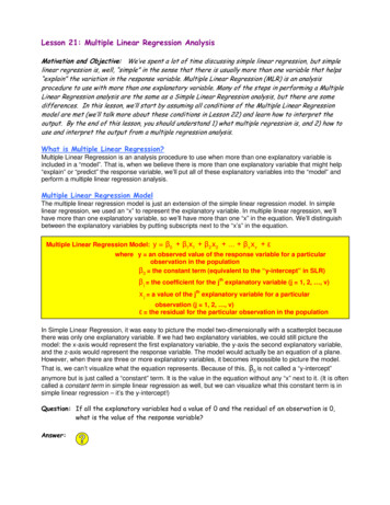
864 Covariance, Regression, and CorrelationTable 4.1 The relationship between the average of both parents (mid parent) and the height of theirchildren. The basic data table is from Galton (1886) who used these data to introduce reversion to themean (and thus, linear regression). The data are available as part of the UsingR or psych packages. Seealso Figures 4.1 and 4.2. library(psych)data(galton)galton.tab - .tab)),decreasing TRUE),] #sort it by decreasing row valueschildparent 61.7 62.2 63.2 64.2 65.2 66.2 67.2 68.2 69.2 70.2 71.2 72.2 73.2 .5114415502000006410241221100000medians. When this is done, it is quite clear that a line goes through most of the medians,with the exception of the two highest values.2A finding that is quite clear is that there is a “reversion to mediocrity” Galton (1877,1886). That is, parents above or below the median tend to have children who are closer tothe median (reverting to mediocrity) than they. But this reversion is true in either direction,for children who are exceptionally tall tend to have parents who are closer to the medianthan they. Now known as regression to the mean, misunderstanding this basic statisticalphenomena has continued to lead to confusion for the past century Stigler (1999). To showthat regression works in both directions Galton’s data are also plotted for child regressed onmid parent (left hand panel) or the middle parent height regressed on the child heights (righthand panel of Figure 4.2.Galton’s solution for finding the slope of the line was graphical although his measure ofreversion, r, was expressed as a reduction in variation. Karl Pearson, who referred to Galton’sfunction later gave Galton credit as developing the equation we now know as the PearsonProduct Moment Correlation Coefficient Pearson (1895, 1920).Galton recognized that the prediction equation for the best estimate of Y, Ŷ , is merelythe solution to the linear equationŶ by.x X c(4.1)which, when expressed in deviations from the mean of X and Y, becomesŷ by.x x.2(4.2)As discussed by Wachsmuth et al. (2003), this bend in the plot is probably due to the way Galtoncombined male and female heights.
4 Covariance, Regression, and Correlation8774Galton's regression 626466687072 Child Height 6466 6870 72Mid Parent HeightFig. 4.1 The data in Table 4.1 can be plotted to show the relationships between mid parent and childheights. Because the original data are grouped, the data points have been jittered to emphasize thedensity of points along the median. The bars connect the first, 2nd (median) and third quartiles. Thedashed line is the best fitting linear fit, the ellipses represent one and two standard deviations fromthe mean.The question becomes one of what slope best predicts Y or y. If we let the residual ofprediction be e y ŷ, then Ve , the average squared residualfunction of by.x :nnnni 1i 1i 1i 1n e2 /n, will be a quadratici 1Ve e2 /n (y ŷ)2 /n (y by.x x)2 /n (y2 2by.x xy b2y.x x2 )/n(4.3)Ve is minimized when the first derivative with respect to b of equation 4.3 is set to 0.nd(Ve ) (2xy 2by.x x2 )/n 2Covxy 2bσx2 0d(b)i 1which implies thatby.x Covxy.σx2(4.4)(4.5)That is, by.x , the slope of the line predicting y given x that minimizes the squared residual(also known as the squared error of prediction) is the ratio of the Covariance between x andy and the Variance of X. Similarly, the slope of the line that best predicts x given values ofy will beCovxybx.y .(4.6)σy2
884 Covariance, Regression, and Correlation74Mid parent child74Child mid parent 6872 70 68Mid Parent Height70 66Child Height 6672 6464 b 0.336262b 0.656264666870Mid Parent Height727462646668707274Child HeightFig. 4.2 Galton (1886) examined the relationship between the average height of parents and theirchildren. He corrected for sex differences in height by multiplying the female scores by 1.08, and thenfound the average of the parents (the mid parent). Two plots are shown. The left hand panel showschild height varying as the mid parent height. The right hand panel shows mid parent height varyingas child height. For both panels, the vertical lines and bars show the first, second (the median), andthird interpolated quartiles. The slopes of the best fitting lines are given (see Table 4.2). Galton wasaware of this difference in slopes and suggested that one should convert the variability of both variablesto standard units by dividing the deviation scores by the inter-quartile range. The non-linearity in themedians for heights about 72 inches is discussed by Wachsmuth et al. (2003)As an example, consider the galton data set, where the variances and covariances are foundby the cov function and the slopes may be found by using the linear model function lm(Table 4.2). There are, of course two slopes: one for the best fitting line predicting the heightof the children given the average (mid) of the two parents and the other is for predicting theaverage height of the parents given the height of their children. As reported by Galton, thefirst has a slope of .65, the second a slope of .33. Figure 4.2 shows these two regressions andplots the median and first and third quartiles for each category of height for either the parents(the left hand panel) or the children (the right hand panel). It should be noted how well thelinear regression fits the median plots, except for the two highest values. This non-linearityis probably due to the way that Galton pooled the heights of his male and female subjects(Wachsmuth et al., 2003).4.1 Correlation as the geometric mean of regressionsGalton’s insight was that if both x and y were on the same scale with equal variability, thenthe slope of the line was the same for both predictors and was measure of the strength of theirrelationship. Galton (1886) converted all deviations to the same metric by dividing through
4.1 Correlation as the geometric mean of regressions89Table 4.2 The variance/covariance matrix of a data matrix or data frame may be found by using thecov function. The diagonal elements are variances, the off diagonal elements are covariances. Linearmodeling using the lm function finds the best fitting straight line and cor finds the correlation. All threefunctions are applied to the Galton dataset galton of mid parent and child heights. As was expectedby Galton (1877), the variance of the mid parents is about half the variance of the children, the slopepredicting child as a function of mid parent is much steeper than that of predicting mid parent fromchild. The cor function finds the covariance for standardized scores. data(galton)cov(galton)lm(child parent,data galton)lm(parent child,data galton)round(cor(galton),2)parentchildparent 3.194561 2.064614child 2.064614 6.340029Call:lm(formula child parent, data Call:lm(formula parent child, data hild0.3256parent child1.00 0.460.46 1.00by half the interquartile range, and Pearson (1896) modified this by converting the numbersto standard scores (i.e., dividing the deviations by the standard deviation). Alternatively, thegeometric mean of the two slopes (bx y and by x) leads to the same outcome: (CovxyCovyxCovxyCovxyrxy bxy byx (4.7)22σx σyσx σyσ 2σ 2xywhich is the same as the covariance of the standardized scores of X and Y.rxy Covzx zy Covx yσx σy Covxyσx σy(4.8)
904 Covariance, Regression, and CorrelationIn honor of Karl Pearson (1896), equation 4.8, which expresses the correlation as the productof the two standardized deviation scores, or the ratio of the moment of dynamics to thesquare root of the product of the moments of inertia, is known as the Pearson Product Moment Correlation Coefficient. Pearson (1895, 1920), however, gave credit for the correlationcoefficient to Galton (1877) and used r as the symbol for correlation in honor of Galton’sfunction or the coefficient of reversion. Correlation is done in R using the cor function, aswell as rcorr in the Hmisc package. Tests of significance (see section 4.4.1) are done using cor.test. Graphic representations of correlations that include locally smoothed linearfits (lowess regressions) are shown in the pairs or in the pairs.panels functions. For thegalton data set, the correlation is .46 (Table 4.2).Fig. 4.3 Scatter plots of matrices (SPLOMs) are very useful ways of showing the strength of relationships graphically. Combined with locally smoothed regression lines (lowess), histograms and densitycurves, and the correlation coefficient, SPLOMs are very useful exploratory summaries. The data arefrom the sat.act data set in psych.5 10200400600800 ACT 200.11 0.04 0.034060300.56 0.595152535age20 200400600800 203040 5060 0.64 SATV 600 400 200 800 SATQ 2004006008004.2 Regression and predictionThe slope by.x was found so that it minimizes the sum of the squared residual, but what isit? That is, how big is the variance of the residual? Substituting the value of by.x found inEq 4.6 into Eq 4.3 leads to
4.3 A geometric interpretation of covariance and correlation91nnnni 1i 1i 1i 1Vr r2 /n (y ŷ)2 /n (y by.x x)2 /n (y2 b2y.x x2 2by.x xy)/nVr Vy b2y.xVx 2by.xCovxy Vy Vr Vy Cov2xyCovxyVx 2CovxyVx2VxCov2xyCov2xyCov2xy 2 Vy VxVxVx22Vr Vy rxyVy Vy (1 rxy)(4.9)That is, the variance of the residual in Y or the variance of the error of prediction of Y isthe product of the original variance of Y and one minus the squared correlation between Xand Y. This leads to the following table of relationships:Table 4.3 The basic relationships between Variance, Covariance, Correlation and ResidualsVariance Covariance with X Covariance with Y Correlation with X Correlation with YXVxVxCxy1rxyYVyCxyVyrxy12VŶrxyCxy rxy σx σyrxyVy1rxyy 2 )V2 )VYr Y Ŷ (1 rxy0(1 rxy01 r2yy4.3 A geometric interpretation of covariance and correlationBecause X and Y are vectors in the space defined by the observations, the covariance betweenthem may be thought of in terms of the average squared distance between the two vectorsin that same space (see Equation 3.14). That is, following Pythagorus, the distance, d, issimply the square root of the sum of the squared distances in each dimension (for each pairof observations), or, if we find the average distance, we can find the square root of the sumof the squared distances divided by n: 1 ndxy (xi yi )2n i 1or2dxy which is the same as1 n (xi yi )2 .n i 12dxy Vx Vy 2Cxybut becauserxy Cxyσx σy2dxy σx2 σy2 2σx σy rxy(4.10)
924 Covariance, Regression, and Correlationordxy 2 (1 rxy ).(4.11)Compare this to the trigonometric law of cosines,c2 a2 b2 2ab · cos(ab),and we see that the distance between two vectors is the sum of their variances minus twicethe product of their standard deviations times the cosine of the angle between them. Thatis, the correlation is the cosine of the angle between the two vectors. Figure 4.4 shows theserelationships for two Y vectors. The correlation, r1 , of X with Y1 is the cosine of θ1 the ratioof the projection of Y1 onto X. From the Pythagorean Theorem, the length of the residual Ywith X removed (Y.x) is σy 1 r2 .1 r22y2y10.0θ21 r21θ1 r2r1 1.0 0.5Residual0.51.0Correlations as cosines 1.0 0.50.00.51.0XFig. 4.4 Correlations may be expressed as the cosines of angles between two vectors or, alternatively,the length of the projection of a vector of length one upon another. Here the correlation between X andY1 r1 cos(θ1 ) and the correlation between X and Y2 r2 cos(θ2 ). That Y2 has a negative correlationwith X means that unit change in X lead to negative changes in Y. The vertical dotted lines representthe amount of residual in Y, the horizontal dashed lines represent the amount that a unit change in Xresults in a change in Y.
4.4 The bivariate normal distribution93Linear regression is a way of decomposing Y into that which is predicable by X and thatwhich is not predictable (the residual). The variance of Y is merely the sum of the variancesof bX and residual Y. If the standard deviation of X, Y, and the residual Y are thought ofas the length of their respective vectors, then the sin of the angle between X and Y is VVyrand the vector of length 1 Vr is the projection of Y onto X. (Refer to Table 4.3).4.4 The bivariate normal distributionIf x and y are both continuous normally distributed variables with mean 0 and standarddeviation 1, then the bivariate normal distribution isf (x) 21(2π(1 r2 )2x 2x x x 1 1 22 2e2(1 r ).(4.12)The mvtnorm and MASS packages provides functions to find the cumulative density function, probability density function, or to generate random elements from the bivariate normaland multivariate normal and t distributions (e.g., rmvnorm and mvrnorm).4.4.1 Confidence intervals of correlationsFor a given correlation, rxy , estimated from a sample size of n observations and with theassumption of bivariate normality, the t statistic with degrees of freedom, d f n 2 may beused to test for deviations from 0 (Fisher, 1921). r n 2td f (4.13)1 r2Although Pearson (1895) showed that for large samples, that the standard error of r was(1 r2 ) n(1 r2 )Fisher (1921) used the geometric interpretation of a correlation and showed that for population value ρ, by transforming the observed correlation r into a z using the arc tangenttransformation:z 1/2 log(1 r)1 rz̄ 1/2 log(1 ρ)1 ρthen z will have a meanwith a standard error of σz 1/ (n 3)(4.14)(4.15)
944 Covariance, Regression, and CorrelationConfidence intervals for r are thus found by using the r to z transformation (Equation 4.14),the standard error of z (Equation 4.15), and then back transforming to the r metric (fisherzand fisherz2r). The cor.test function will find the t value and associated probability valueand the confidence intervals for a pair of variables. The rcorr function from Frank Harrell’sHmisc package will find Pearson or Spearman correlations for the columns of matrices andhandles missing values by pairwise deletion. Associated sample sizes and p-values are reportedfor each correlation. The r.con function from the psych package will find the confidenceintervals for a specified correlation and sample size (Table 4.4).Table 4.4 Because of the non-linearity of the r to z transformations, and particularly for large valuesof the estimated correlation, the confidence interval of a correlation coefficient is not symmetric aroundthe estimated value. The two-tailed p values in the following table are based upon the t-test for adifference from 0 with a sample size of 30 and are found using the pt function. The t values are founddirectly from equation 4.13 by the r.con function. n - 30r - seq(0,.9,.1)rc - matrix(r.con(r,n),ncol 2)t - r*sqrt(n-2)/sqrt(1-r 2)p - (1-pt(t,n-2))/2r.rc - data.frame(r r,z fisherz(r),lower rc[,1],upper rc[,2],t t,p wer uppert-0.36 0.36 0.00-0.27 0.44 0.53-0.17 0.52 1.08-0.07 0.60 1.660.05 0.66 2.310.17 0.73 3.060.31 0.79 3.970.45 0.85 5.190.62 0.90 7.060.80 0.95 10.93p0.250.150.070.030.010.000.000.000.000.00add z to the table4.4.2 Testing whether correlations differ from zeroNull Hypothesis Significance Tests, NHST , examine the likelihood of observing a particularcorrelation given the null hypothesis of no correlation. This is may be found by using Fisher’stest (equation 4.13) and finding the probability of the resulting t statistic using the pt functionor, alternatively, directly by using the corr.test function. Simultaneous testing of sets ofcorrelations may be done by the rcorr function in the Hmisc package.The problem of whether a matrix of correlations, R, differs from those that would beexpected if sampling from a population of all zero correlations was addressed by Bartlett(1950, 1951) and Box (1949). Bartlett showed that a function of the natural logarithm of thedeterminant of a correlation matrix, the sample size (N), and the number of variables (p) isasymptotically distributed as χ 2 :
4.4 The bivariate normal distribution95χ 2 ln R (N 1 (2p 5)/6)(4.16)with degrees of freedom, d f p (p 1)/2. The determinant of an identity matrix is one, andas the correlations differ from zero, the determinant will tend towards zero. Thus Bartlett’stest is a function of how much the determinant is less than one. This may be found by thecortest.bartlett function. Given that the standard error of a z transformed correlation is 1/ n 3, and that asquared z scores is χ 2 , a very reasonable alternative is to consider whether the sum of thesquared correlations differs from zero. When multiplying this sum by n-3, this is distributedas χ 2 with p*(p-1)/2 degrees of freedom. This is a direct test of whether the correlationsdiffer from zero Steiger (1980c). This test is available as the cortest function.4.4.3 Testing the difference between correlationsThere are four different tests of correlations and the differences between correlations thatare typically done: 1) is a particular correlation different from zero, 2) does a set of ofcorrelations differ from zero, 3) do two correlations (taken from different samples) differ fromeach other, and 4) do two correlations taken from the same sample differ from each other.The first question, does a correlation differ from zero was addressed by Fisher (1921) andanswered using a t-test of the observed value versus 0 (Equation 4.13) and looking up theprobability of observing that size t or larger with degrees of freedom of n-2 with a call to pt(see Table 4.4 for an example). The second is answered by applying a χ 2 test (equation 4.16)using either the cortest.bartlett or cortest functions. The last two of these questionsare more complicated and have two different sub questions associated with them.Olkin and Finn (1990, 1995) and Steiger (1980a) provide very complete discussion andexamples of tests of the differences between correlations as well as the confidence intervals forcorrelations and their differences. Three of the Steiger (1980a) tests are implemented in ther.test function in the psych package. Olkin and Finn (1995) emphasize confidence intervalsfor differences between correlations and address the problem of what variable to choose whenadding to a multiple regression.4.4.3.1 Testing independent correlations: r12 is different from r34To test two whether two correlations are different involves a z-test and depends upon whetherthe correlations are from different samples or from the same sample (the dependent or correlated case). In the first case, where the correlations are independent, the correlations aretransformed to zs and the test is just the ratio of the differences (in z units) compared tothe standard error of a difference. The standard error is merely the square root of the sumof the squared standard errors of the two individual correlations:which is the same aszr12 zr34zr12 r34 1/(n1 3) 1/(n2 3)zr12 r34 1 r34121/2 log( 1 r1 r12 ) 1/2 log( 1 r34 ) .1/(n1 3) 1/(n2 3)(4.17)
964 Covariance, Regression, and CorrelationThis seems more complicated than it really is and can be done using the paired.r or r.testfunctions (Table 4.5).Table 4.5 Testing two independent correlations using Equation 4.17 and r.test results in a z-test. r.test(r12 .25,r34 .5,n 100) test[1] "test of difference between two independent correlations" z[1] 2.046730 p[1] 0.040684584.4.3.2 Testing dependent correlations: r12 is different from r23A more typical test would be to examine whether two variables differ in their correlationwith a third variable. Thus with the variables X1 , X2 , and X3 with correlations r12 , r13 and r23the t of the difference of r12 minus r13 is (n 1) (1 r23 )(4.18)tr12 r13 (r12 r13 ) (n 1)13 232 n 3 R r12 r(1 r)232where R is the determinant of the 3 *3 matrix of correlations and is222 R 1 r12 r13 r12 2 r12 r13 r23(4.19)(Steiger, 1980a). Consider the case of Extraversion, Positive Affect, and Energetic Arousalwith PA and EA assessed at two time points with 203 participants (Table 4.6). The t forthe difference between the correlations of Extraversion and Positive Affect at time 1 (.6)and Extraversion and Energetic Arousal at time 1 (.5) is found from equation 4.18 usingthe paired.r function and is 1.96 with a p value .05. Steiger (1980a) and Dunn andClark (1971) argue that Equation 4.18, Williams’ Test (Williams, 1959), is preferred toan alternative test for dependent correlations, the Hotelling T , which although frequentlyrecommended, should not be used.4.4.3.3 Testing dependent correlations: r12 is different from r34Yet one more case is the test of equality of two correlations both taken from the samesample but for different variables (Steiger, 1980a). An example of this would be whether thecorrelations for Positive Affect and Energetic Arousal at times 1 and 2 are the same. For fourvariables (X1 .X4 ) with correlations r12 .r34 , the z of the difference of r12 minus r34 is (z12 z34 ) n 3zr12 r34 (4.20)2(1 r12,34 )
4.4 The bivariate normal distribution97Table 4.6 The difference between two dependent correlations, rext,PA1 and rext,EA1 is found using Equation 4.18 which is implement in the paired.r and r.test functions. Because these two correlationsshare a common element (Extraversion), the appropriate test is found in Equation 4.18.ExtraversionPositive Affect 1Energetic Arousal 1Positive Affect 2Energetic Arousal 2Ext 1 PA 1 EA 1 PA 2 EA 21.61.5.61.4.8.61.3.6.8.51 r.test(r12 .6,r13 .5,r23 .6,n 203)Correlation testsCall:r.test(n 203, r12 0.6, r23 0.6, r13 0.5)Test of difference between two correlated correlationst value 2with probability 0.047wherer12,34 1/2([(r13 r12 r23 )(r24 r23 r34 )] [(r14 r13 r34 )(r23 r12 r13 )] [(r13 r14 r34 )(r24 r12 r14 )] [(r14 r12 r24 )(r23 r24 r34 )])reflects that the correlations themselves are correlated. Under the null hypothesis of equivalence, we can also assume that the correlations r12 r34 (Steiger, 1980a) and thus both ofthese values can be replaced by their averager12 r34 r12 r34.2Calling r.test with the relevant correlations strung out as a vector shows that indeed, thetwo correlations (.6 and .5) do differ reliably with a probability of .04 (Table 4.7).Table 4.7 Testing the difference between two correlations from the same sample but that do notoverlap in the variables included. Because the correlations do not involve the same elements, but doinvolve the same subjects, the appropriate test is Equation 4.20. r.test(r12 .6,r34 .5,r13 .8,r14 .6,r23 .6,r24 .8,n 203)Correlation testsCall:r.test(n 203, r12 0.6, r34 0.5, r23 0.6, r13 0.8, r14 0.6,r24 0.8)Test of difference between two dependent correlationsz value 2.05with probability 0.04
984 Covariance, Regression, and Correlation4.4.3.4 Testing whether correlation matrices differ across groupsThe previous tests were comparisons of single correlations. It is also possible to test whetherthe observed p * p correlation matrix, R1 for one group of subje
88 4 Covariance, Regression, and Correlation 62 64 66 68 70 72 74 62 64 66 68 70 72 74 Mid Parent Height Child Height Child mid parent