Transcription
Exact ray tracing in MATLABMaria Ruiz-GonzalezIntroductionThis tutorial explains how to program a simple geometric ray tracing program in MATLAB, which can bewritten in any other programming language like C or Python and extended to add elements andcomplexity. The main purpose is that the student understands what a ray tracing software like Zemax orCode V does, and that the analysis can be performed even if there’s no access to any of those software.The code consists of a main program and a function for a plano-convex lens that in turn consists of anothertwo functions, one for the refraction at a spherical surface and a second one for refraction at a planesurface, as explained in figure 1. Building the program in functions makes easier to debug and understandsince the code is simpler, and since each surface is a different function, different elements can be easilyconstructed.By using a for-loop, it is possible to compute many different rays at the same time, which are stored inthe rows of a matrix. That matrix has all the information necessary to perform different analyses. Theinputs for the plano-convex lens function are the height of the ray, refractive index, thickness of lens,radius of spherical surface, and resolution for computations in the z-axis. The output is a ray matrix andsome vectors related to the z-axis that make easier the visualization of the results.Finally, two examples of what can be analyzed with the ray matrix are given, that consists of a few extralines of code. It is important to notice that even if we choose to do paraxial optics for simplicity for a firstorder approximation of an optical system, an exact ray trace is also simple and gives us substantially moreinformation, for instance, spherical aberration and ray fan plots.Main program:System analysisFunction:Plano convex lensFunction:Refraction at spherical surfaceFunction:Refraction at plane surfaceFigure 1. Structure of the geometric ray tracing program for a plano-convex lens.
Refraction at plane interfaceThe refraction at an interface is described by the Snell’s law:𝑛 sin 𝜃 𝑛′ sin 𝜃′Figure 2. Refraction at a plane interface described by Snell’s law.The Matlab function for refraction at a plane interface takes as input height y of the ray at the interface,slope 𝑢 tan 𝜃, thickness of the lens, index of refraction n, and vector z, which is used to plot the ray inair (back of lens). In our case, the ray travels from the medium to air.function [ray air] plane refract ray(y,slope,thickness,n,z)theta1 atan(slope);theta2 asin(n*sin(theta1));slope2 tan(theta2);ray air (z-thickness)*slope2 y;end
Refraction at spherical interfaceWe need to compute the slope 𝑢 tan 𝜃 inside the lens, using the geometry in figure 3.Figure 3. Refraction of incoming ray at spherical interface.It is easy to see that:sin 𝜙 𝑦𝑟By Snell’s law:𝑛 sin 𝜙′ sin 𝜙 sin 𝜙′ sin 𝜙𝑛Finally, after some simple geometry:𝜃 𝜙′ 𝜙For the Matlab function, input variables are height y, radius r, thickness of the lens, index of refraction nand step size Δz. Outputs are the ray inside the lens, slope and z axis. In this case, the ray travels from airto the medium.function [ray,slope,z] sphere refract ray(y,radius,thickness,n,dz)sag radius - sqrt(radius 2 - y 2); %lens sag at yz sag:dz:thickness;sin phi1 y/radius;sin phi2 sin phi1/n;phi1 asin(sin phi1);phi2 asin(sin phi2);theta phi2-phi1;slope tan(theta);ray slope*(z-sag) y; % Ray in lensend
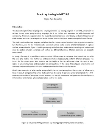
Plano-convex lensFigure 4. Geometry of the plano-convex lens solved in this tutorial.In order to construct the rays through the lens, we have to use the two functions described above, in thecorrect order. The paraxial focal length is computed for visualization purposes. The function for the planoconvex lens takes as input the index of refraction of the lens, radius of first surface, thickness of lens, stepsize Δz and height y. The results for all rays are stored in a matrix, where each row is one ray.function [raymatrix,z front,z optaxis,zmax] plano convex(n,radius,thickness,dz,y)power (n-1)/radius; %lens powerf 1/power; %paraxial focal lengthzmax floor(f .1*f); %end of z-axisz front 0:dz:thickness-dz; %z-axis back of plane surfacez back thickness:dz:zmax-dz; %z-axis front of plane surfacez optaxis [z front,z back]; %total optical axisy(y 0) 10 -10;raymatrix zeros(length(y),length(z optaxis));%Ray tracingfor i 1:length(y)%Refraction at spherical surface[ray lens, slope, x lens] sphere refract ray(y(i),radius,thickness,n,dz);%Refraction at plane surface[ray air] plane refract ray(ray lens(end),slope,thickness,n,z back);%Incoming rayx front air 0:dz:x lens(1)-dz;ray front air y(i)*ones(1,length(x front air));%Create matrix of rays (adjust length if necessary)if length(ray lens) length(ray air) length(x front air) length(z optaxis)raymatrix(i,:) [ray front air,ray lens,ray air];elseraymatrix(i,:) [ray front air, ray lens(1:length(ray lens)-1), ray air];endendend
Main programThe main program is where all the analysis is performed using the information of the height of each rayat all points obtained with the plano-convex lens function. It’s here where the programmer can decidewhat to visualize and the analyses to perform. The example shown here is for a plano-convex lens of radiusR 20 mm, center thickness 2 mm and index of refraction n 1.5168. The next few lines of code are theinitialization variables and the visualization of the system.n 1.5168; %Index of refraction of lensradius 20; %Radius of spherical surfacethickness 2; %Central thickness of lensdz 0.01; %Step size for computation purposesaperture 5;number rays 11;dy (2*aperture 1)/number rays;y -aperture:dy:aperture; %Field of view%Ray matrix[raymatrix,x front,x optaxis,zmax] plano convex(n,radius,thickness,dz,y);%Figurefront lens sqrt(radius 2 - (x front-radius). 2);figure(1)plot(x optaxis,raymatrix','r') %Rayshold on% Lens back surfaceline([thickness thickness], [max(front lens) -max(front lens)],'color','b')plot(x front,front lens,'b',x front,-front lens,'b') %Lens front surfaceplot(x optaxis,zeros(1,length(x optaxis)),'k--') %Optical axishold offaxis([-thickness zmax -max(front lens) max(front lens)])Figure 5. Lens computed with the plano-convex lens function and ray traces forcollimated incoming rays.
Example: Ray fan plotEach column of the ray matrix corresponds to the heights y of all rays at a constant z. In order to computea ray fan plot, we need to find where the paraxial ray crosses the optical axis, and plot the columncorresponding to that point.%Find where each ray crosses optical axisray focus zeros(1,length(y));for i 1:length(y)[a, ray focus(i)] min(abs(raymatrix(i,:)));End%Find where paraxial ray crosses optical axisparaxial focus ray focus(ceil(length(y)/2));%Ray fan plotplot(y,raymatrix(:,paraxial focus)')Figure 6. Ray fan plot for the plano-convex lens.
Example: Longitudinal spherical aberrationIn the previous example, it was found where the rays cross the optical axis. We can plot those values tosee the longitudinal spherical aberration of the system.spher ab x optaxis(ray focus(find(y 0)));plot(spher ab - spher ab(1),y(find(y 0)))Figure 7. Longitudinal spherical aberration of the plano-convex lens.
Appendix ACode to obtain the results presented in this tutorial. Save each function in different files, thename of the file must be the name of the function, e.g. sphere refract ray.m.function [ray,slope,z] sphere refract ray(y,radius,thickness,n,dz)sag radius - sqrt(radius 2 - y 2); %lens sag at yz sag:dz:thickness;sin phi1 y/radius;sin phi2 sin phi1/n;phi1 asin(sin phi1);phi2 asin(sin phi2);theta phi2-phi1;slope tan(theta);ray slope*(z-sag) y; % Ray in lensendfunction [ray air] plane refract ray(y,slope,thickness,n,z)theta1 atan(slope);theta2 asin(n*sin(theta1));slope2 tan(theta2);ray air (z-thickness)*slope2 y;endfunction [raymatrix,z front,z optaxis,zmax] plano convex(n,radius,thickness,dz,y)power (n-1)/radius; %lens powerf 1/power; %paraxial focal lenghtzmax floor(f .1*f);z front 0:dz:thickness-dz; %x-axis back of plane surfacez back thickness:dz:zmax-dz; %x-axis front of plane surfacez optaxis [z front,z back]; %total optical axisy(y 0) 10 -10;raymatrix zeros(length(y),length(z optaxis));%Ray tracingfor i 1:length(y)%Refraction at spherical surface[ray lens, slope, x lens] sphere refract ray(y(i),radius,thickness,n,dz);%Refraction at plane surface[ray air] plane refract ray(ray lens(end),slope,thickness,n,z back);%Ray comming inx front air 0:dz:x lens(1)-dz;ray front air y(i)*ones(1,length(x front air));%Create matrix of rays (adjust length if necessary)if length(ray lens) length(ray air) length(x front air) length(z optaxis)raymatrix(i,:) [ray front air,ray lens,ray air];elseraymatrix(i,:) [ray front air, ray lens(1:length(ray lens)-1), ray air];endendend
%% Plano-convex lens: ray tracing analysisclear alln 1.5168; %Index of refraction of lensradius 20; %Radius of spherical surfacethickness 2; %Central thickness of lensdz 0.01; %Step size for computation purposes%dy 1; %Separation between raysaperture 5;number rays 11;dy (2*aperture 1)/number rays;y -aperture:dy:aperture; %Field of view%Ray matrix[raymatrix,x front,x optaxis,zmax] plano convex(n,radius,thickness,dz,y);%Figuresfront lens sqrt(radius 2 - (x front-radius). 2);figure(1)plot(x optaxis,raymatrix','r') %Rayshold online([thickness thickness], [max(front lens) -max(front lens)],'color','b')%Lens back surfaceplot(x front,front lens,'b',x front,-front lens,'b') %Lens front surfaceplot(x optaxis,zeros(1,length(x optaxis)),'k--') %Optical axishold offaxis([-thickness zmax -max(front lens) max(front lens)])%% Ray fan plots%Find where each ray focusesray focus zeros(1,length(y));for i 1:length(y)[a, ray focus(i)] min(abs(raymatrix(i,:)));end%Find where paraxial ray focusesparaxial focus ray focus(ceil(length(y)/2));figure(2)%Ray-fan plotplot(y,raymatrix(:,paraxial focus)')%% Spherical aberrationfigure(3)spher ab x optaxis(ray focus(find(y 0)));plot(spher ab - spher ab(1),y(find(y 0)))
This tutorial explains how to program a simple geometric ray tracing program in MATLAB, which can be written in any other programming language like C or Python and extended to add elements and complexity. The main purpose is that the student understands what a ray tracing software like Zemax or Code V does, and that the analysis can be .