Transcription
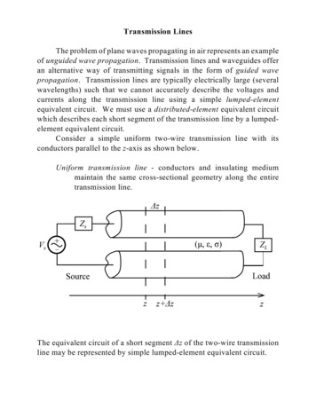
Transmission LinesThe problem of plane waves propagating in air represents an exampleof unguided wave propagation. Transmission lines and waveguides offeran alternative way of transmitting signals in the form of guided wavepropagation. Transmission lines are typically electrically large (severalwavelengths) such that we cannot accurately describe the voltages andcurrents along the transmission line using a simple lumped-elementequivalent circuit. We must use a distributed-element equivalent circuitwhich describes each short segment of the transmission line by a lumpedelement equivalent circuit.Consider a simple uniform two-wire transmission line with itsconductors parallel to the z-axis as shown below.Uniform transmission line - conductors and insulating mediummaintain the same cross-sectional geometry along the entiretransmission line.The equivalent circuit of a short segment Äz of the two-wire transmissionline may be represented by simple lumped-element equivalent circuit.
R series resistance per unit length (Ù/m) of the transmission lineconductors.L series inductance per unit length (H/m) of the transmission lineconductors (internal plus external inductance).G shunt conductance per unit length (S/m) of the media betweenthe transmission line conductors.C shunt capacitance per unit length (F/m) of the transmission lineconductors.We may relate the values of voltage and current at z and z Äz bywriting KVL and KCL equations for the equivalent circuit.KVLKCL
Grouping the voltage and current terms and dividing by Äz givesTaking the limit as Äz 6 0, the terms on the right hand side of the equationsabove become partial derivatives with respect to z which givesTime-domaintransmission lineequations(coupled PDE’s)For time-harmonic signals, the instantaneous voltage and current may bedefined in terms of phasors such thatThe derivatives of the voltage and current with respect to time yield jùtimes the respective phasor which givesFrequency-domain(phasor) transmissionline equations(coupled DE’s)Note the similarity in the functional form of the time- and frequencydomain transmission line equations to the respective source-free Maxwell’sequations (curl equations). Even though these equations were derivedwithout any consideration of the electromagnetic fields associated with thetransmission line, remember that circuit theory is based on Maxwell’sequations.
Given the similarity of the phasor transmission line equations toMaxwell’s equations, we find that the voltage and current on a transmissionline satisfy wave equations. These voltage and current wave equations arederived using the same techniques as the electric and magnetic field waveequations. Beginning with the phasor transmission line equations, we takederivatives of both sides with respect to z.We then insert the first derivatives of the voltage and current found in theoriginal phasor transmission line equations.The voltage and current wave equations may be written aswhere ã is the complex propagation constant of the wave on thetransmission line given by
Just as with unguided waves, the real part of the propagation constant (á)is the attenuation constant while the imaginary part (â) is the phaseconstant. The general equations for á and â in terms of the per-unit-lengthtransmission line parameters areThe general solutions to the voltage and current wave equations are z-directed waves a!z-directed wavesThe current equation may be written in terms of the voltage coefficientsthrough the original phasor transmission line equations.The complex constant Z o is defined as the transmission line characteristicimpedance and is given by
The transmission line equations written in terms of voltage coefficientsonly areThe complex voltage coefficients may be written in terms of magnitude andphase asThe instantaneous voltage becomesThe wavelength and phase velocity of the waves on the transmission linemay be found using the points of constant phase as was done for planewaves.
Lossless Transmission LineIf the transmission line loss is neglected (R G 0), the equivalentcircuit reduces toNote that for a true lossless transmission line, the insulating mediumbetween the conductors is characterized by a zero conductivity (ó 0), andreal-valued permittivity å and permeability ì (åO ìO 0). Thepropagation constant on the lossless transmission line isGiven the purely imaginary propagation constant, the transmission lineequations for the lossless line are
The characteristic impedance of the lossless transmission line is purely realand given byThe phase velocity and wavelength on the lossless line areExample (Lossless coaxial transmission line)The dominant mode on a coaxial transmission line is the TEM(transverse electromagnetic) mode defined by E z H z 0. Due to thesymmetry of the coaxial transmission line, thetransverse fields are independent of ö. Thus,we may writeBetween the conductors, the fields mustsatisfy the source-free Maxwell’s equations:
The field components E ñ and H ö are related to the transmission line voltageand current byIf we integrate the Faraday’s law equation along the path C 1 and integratethe Ampere’s law equation along the path C 2,which are the lossless transmission line equations.Terminated Lossless Transmission LineIf we choose our reference point (z 0) at the load termination, thenthe lossless transmission line equations evaluated at z 0 give the loadvoltage and current.
The ratio of voltage to current at z 0 must equal the load impedance.Solving this equation for the voltage coefficient of the !z traveling wavegiveswhere à is the reflection coefficient which defines the ratio of the reflectedwave to the incident wave.Note that the reflection coefficient is in general complex with 0 # *Ã*# 1.If the reflection coefficient is zero (Z L Z o), there is no reflected wave andthe load is said to be matched to the transmission line. If Z L Z o, themagnitude of the reflection coefficient is non-zero (there is a reflectedwave). The presence of forward and reverse traveling waves on thetransmission line produces standing waves.We may rewrite the transmission line equations in terms of thereflection coefficient asor
The magnitude of the transmission line voltage may be written asThe maximum and minimum voltage magnitudes areThe ratio of maximum to minimum voltage magnitudes defines thestanding wave ratio (s).Note that the standing wave ratio is real with 1 # s # 4.
The time-average power at any point on the transmission line is given by Purely imaginaryA ! A * 2j Im{A}P i incident powerP r reflected powerThe return loss (RL) is defined as the ratio of incident power to reflectedpower. The return loss in dB is
Matched load*Ã* 0s 1RL 4 (dB)Total reflection*Ã* 1s 4RL 0 (dB)Transmission Line ImpedanceThe impedance at any point on the transmission line is given by
The impedance at the input of a transmission line of length l terminatedwith an impedance Z L isLossless Transmission Line with Matched Load (Z L Z o)Note that the input impedance of the lossless transmission line terminatedwith a matched impedance is independent of the line length. Any mismatchin the transmission line system will cause standing waves and make theinput impedance dependent on the length of the line.
Short-Circuited Lossless Transmission Line (Z L 0)[See Figure 2.6 (p.61)]The input impedance of a short-circuited lossless transmission line is purelyreactive and can take on any value of capacitive or inductive reactancedepending on the line length. The incident wave is totally reflected (withinversion) from the load setting up standing waves with *V*min 0 and*V*max 2*V o *.
Open-Circuited Lossless Transmission Line (Z L 4)[See Figure 2.8 (p.62)]The input impedance of an open-circuited lossless transmission line ispurely reactive and can take on any value of capacitive or inductivereactance depending on the line length. The incident wave is totallyreflected (without inversion) from the load setting up standing waves with*V*min 0 and *V*max 2*V o *.
Transmission Line ConnectionsThe analysis of a connection between two distinct transmission linescan be performed using the same techniques used for plane wavetransmission/reflection at a material interface. Consider two losslesstransmission lines of different characteristic impedances connected asshown below.Assume that a source is connected to transmission line #1 and transmissionline #2 is terminated with a matched impedance (Z L2 Z o2). Transmissionline #1 is then effectively terminated with a load impedance of Z o2 whichconstitutes a mismatch. At the transmission line connection, a portion ofthe incident wave on transmission line #1 is transmitted onto transmissionline #2 while the remainder is reflected back on transmission line #1. Thus,we may write the voltages on the two transmission lines aswhere à is the reflection coefficient on transmission line #1 and T is thetransmission coefficient on transmission line #2. Equating the voltages atthe transmission line connection point (z 0) gives
Note the similarity between the equations for plane wave (unguided wave)transmission/reflection at a material interface and the guided wavetransmission/reflection at a transmission line connection.Insertion LossStrictly speaking, insertion loss is the ratio of power absorbed by aload before and after a network is inserted into the line. For the previousexample connection between two transmission lines, we consider thematched case for transmission line #1 and the case with transmission line#2 inserted into the system.The insertion loss (IL) is then
Smith ChartThe Smith chart is a useful graphical tool used to calculate thereflection coefficient and impedance at various points on a transmissionline system. The Smith chart is actually a polar plot of the complexreflection coefficient Ã(z) overlaid with the corresponding impedance Z(z).The voltage at any point on the transmission line isThe reflection coefficient at any point on the transmission line is definedaswhere à is the reflection coefficient at the load (z 0).Smith chart center Y *Ã* 0(no reflection - matched)Outer circle Y *Ã* 1(total reflection)
The reflection coefficient for a lossless transmission line of characteristicimpedance Z o, terminated with an impedance Z L is given by(1)where zL is the normalized load impedance. If we solve (1) for z L, we find(2)where rL and x L are the normalized load resistance and reactance,respectively. Equation (2) shows that the reflection coefficient on theSmith chart corresponds to a specific normalized load impedance for thegiven transmission line / load combination. Solving (2) for the resistanceand reactance gives equations for the “resistance” and “reactance” circles:
In a similar fashion, the general impedance at any point along thelength of the transmission line may be written asThe normalized value of the impedance z n(z) is(3)Note the similarity between Equations (2) and (3). The magnitude of thereflection coefficient is constant on a lossless line. Thus, Equation (3)shows that once we locate the normalized load impedance on the Smithchart, we simply rotate through an angle of 2âz on the *Ã* circle to find theimpedance at a given point on the transmission line. Evaluating thereflection coefficient at the transmission line input (z !l ) giveswhich defines a negative phase shift moving toward the generator from theload. Thus, in generalCW rotationYtoward the generatorCCW rotationYtoward the loadOne complete revolution on the Smith chart occurs forThus, each revolution on the Smith chart represents a movement of one-halfwavelength along the transmission line (ë 720 o).Once an impedance point is located on the Smith chart, the equivalentadmittance point is found by rotating 180 o from the impedance point on theconstant reflection coefficient circle.
Example Problem 2.19 (using equations and Smith chart)(b.)(a.)(c.)(d.)(e.)
(f.)
Lossy Transmission LinesThe general transmission line equations (defined in terms of acomplex propagation constant) must be used when dealing with lossy lines.The general transmission line equations areThe reflection coefficient for a lossy transmission line may be determinedby replacing each j â term with ã which givesIn a similar fashion, the input impedance of a terminated lossy transmissionline isMost transmission lines are designed with materials which produce smalllosses (low loss lines). The general expressions for the characteristicimpedance and propagation constant of a lossy transmission line may besimplified somewhat for a low-loss line.
Lossless lineYR G 0Low loss lineYR ùL, G ùCThus, for the equivalent circuit of a low loss line, the reactance terms mustbe much larger than the resistance terms at all frequencies of operation.The general equation for the propagation constant on a lossytransmission line may be approximated as follows for a low loss line.Note that we still include the dominant loss terms (even though they aresmall for a low loss line). Using a Taylor series expansion for the squareroot term above yields
Using the same approximations for the characteristic impedance, we findThe power level delivered to the load is lower than that delivered tothe transmission line input due to the line losses. The line losses can bedetermined by calculating the difference in these power levels. The voltageand current at the load areThe power delivered to the load is
The voltage and current at the input to the transmission line areThe power delivered to the input of the transmission lineThe power lost in the transmission line is
Distortionless Transmission LineOn a lossless transmission line, the propagation constant is purelyimaginary and given byThe phase velocity on the lossless line isNote that the phase constant which varies linearly with frequency producesa constant phase velocity (independent of frequency) so that all frequenciespropagate along the lossless transmission line at the same velocity. FromFourier theory, we know that any time-domain signal may be representedas a weighted sum of sinusoids. Thus, signals transmitted along a losslesstransmission line will suffer no distortion since all of the frequencycomponents propagate at the same velocity. When the phase velocity of atransmission line is a function of frequency, signals will become distortedas different components of the signal arrive at different times. This effectis called dispersion.For the low-loss line, using the appropriate approximations, we foundwhich implies that the phase velocity on a low loss line is near constant.However, the small variations in the phase velocity on a low loss line mayproduce significant distortion if the line is very long.There is a special case of lossy line with the linear phase constant thatproduces a distortionless line. A transmission line is a distortionless lineif the per-unit-length parameters satisfyInserting the per-unit-length parameter relationship into the generalequation for the propagation constant on a lossy line gives
Although the shape of the signal is not distorted, the signal will sufferattenuation as the wave propagates along the line since the distortionlessline is a lossy transmission line. Note that the attenuation constant for adistortionless transmission line is also independent of frequency. If thiswere not true, the signal would suffer distortion due to different frequenciesbeing attenuated by different amounts.In the previous derivation, we have assumed that the per-unit-lengthparameters of the transmission line are independent of frequency. This isalso an approximation that depends on the spectral content of thepropagating signal. For very wideband signals, the attenuation and phaseconstants will, in general, be functions of frequency.For most practical transmission lines, we find that RC GL. In orderto satisfy the distortionless line requirement, series loading coils aretypically placed periodically along the line to increase L.
Perturbation Method for Determining AttenuationGiven only a forward wave propagating along a low loss transmissionline, the voltage and current of the wave may be written asThe power flow as a function of position along the transmission line isgiven by
The power loss per unit length along the transmission line [P l(z)] maybe written asSolving for the attenuation constant givesSince the fields of a low loss transmission line are very close to those of alossless line, we may use the lossless line fields to calculate the power lossper unit length (perturbation method). Note that power P(z) and the powerloss per unit length P l(z) may be evaluated at any point on the transmissionline. The perturbation method allows for the calculation of the attenuationconstant using the transmission line fields rather than using the per-unitlength parameters in the general propagation constant formula.
Example (Perturbation method - coaxial line attenuation constant)The fields within a lossless coaxial line areThe attenuation constant, accordingto the perturbation method, isThe power flow at any point on the transmission line may be found byintegrating the Poynting vector over the surface S where the fields arelocated [S is defined by (a#ñ#b) and (0#ö#2ð)].
Assuming that the dielectric and magnetic losses are negligible, the powerloss per unit length in the conductors of the coaxial line is given bywhere Jsi and Jso are the surface currents on the inner and outer conductorswhile R si and R so are the surface resistances of the inner and outerconductors. The surface S i on the inner conductor is defined by ñ a,0#ö#2ð, and 0#z#l while the surface S o on the outer conductor is definedby ñ b, 0#ö#2ð, and 0#z#l. Using the surface impedance approx-imation,the surface current on a good conductor is approximately that on a PECwhich may be written asThus, we may replace the surface currents in the power loss per unit lengthequation by the surface magnetic fields associated with a lossless coaxialline. The power loss per unit length is thenwhere H ti and H to are the tangential magnetic fields on the surface of theinner and outer conductors. If the inner and outer conductors are the samematerial, thenEvaluation of the integrals in the power loss per unit length expressionyields
The attenuation constant due to conductor loss (á c) on the coaxial linebecomesThe surface resistance (R s) of the conductors is related to the skin depth (ä s)byFor RG-59 coaxial cable (Z o 75 Ù, copper conductors, ó 5.8 10 7 É/m,a 0.292 mm, b 1.854 mm, ì ì o ) at 500 MHz,R s 5.83 10 !3 Ù, á c 0.0245 Np/m
Manufacturers normally specify the transmission line attenuation factor inunits of dB/m as opposed to Np/m. The conversion factor between the twounits is determined below.With á defined in Np/m (á nep), the transmission line voltage attenuation isWith á defined in dB/m (á dB), the transmission line voltage attenuation isEquating the two expressions yieldsFor the RG-59 coaxial line,
Wheeler Incremental Inductance RuleBy noting that the conductor loss in a transmission line can be relatedto the small change in the transmission line inductance due to thepenetration of the fields into the conductors, Wheeler derived an equationfor the transmission line conductor loss in terms of the change in thecharacteristic impedance. The result of the Wheeler incremental inductancerule may be written aswhere is R s the surface resistance of the conductor, Z o is the characteristicimpedance of the transmission line assuming perfect conductors, ç is theintrinsic impedance of the dielectric between the conductors, and l definesthe direction into the conductors. The characteristic impedance of thelossless coaxial transmission line is given byThe derivative term in the attenuation factor expression is
The attenuation factor due to conductor loss in the coaxial transmission linebecomeswhich is identical to the result found using the perturbation method.
Smith Chart The Smith chart is a useful graphical tool used to calculate the reflection coefficient and impedance at various points on a transmission line system. The Smith chart is actually a polar plot of the complex re fle ctio n coeffic ie nt Ã(z) ov er lai d w ith t he corr espon di ng imp edan ce Z (z).