Transcription
Statistics for Engineers Kevin Dunn, .ca/Univariate Data Analysis
Copyright, sharing, and attribution noticeThis work is licensed under the Creative Commons Attribution-ShareAlike 4.0 Unported License. Toview a copy of this license, please visit http://creativecommons.org/licenses/by-sa/4.0/This license allows you:Ito share - to copy, distribute and transmit the work, including print itIto adapt - but you must distribute the new result under the same or similarlicense to this oneIcommercialize - you are allowed to use this work for commercial purposesattribution - but you must attribute the work as follows:III“Portions of this work are the copyright of Kevin Dunn”, or“This work is the copyright of Kevin Dunn”(when used without modification)
We appreciate:Iif you let us know about any errors in the slidesIany suggestions to improve the notesAll of the above can be done by writing tokevin.dunn@mcmaster.caor anonymous messages can be sent to Kevin Dunn athttp://learnche.mcmaster.ca/feedback-questionsIf reporting errors/updates, please quote the current revision number:Please note that all material is provided “as-is” and no liability will be accepted foryour usage of the material.
Univariate data analysis: What we will cover
Usage examples for this sectionICo-worker: Here are the yields from a batch system for the last 3 years (1256 datapoints)IIwhat sort of distribution do the data have?yesterday’s yield was less than 160 g/L, what are the chances of that?IYourself: Using historical failure rate data of the pumps, what is the probabilitythat 3 pumps will fail this month?IManager: does reactor 1 have better final product purity, on average, than reactor2?IColleague: what is the 95% confidence interval for the density of your powderingredient?
References and readingsIAny standard statistics text bookIRecommended: Box, Hunter and Hunter, Statistics for Experimenters, Chapter 2(both 1st and 2nd edition)IWikipedia articles on any term that seems unfamiliar or that you’ve forgottenIHodges and Lehmann, Basic Concepts of Probability and StatisticsIHogg and Ledolter, Engineering StatisticsIMontgomery and Runger, Applied Statistics and Probability for Engineers
Concepts: use this as a checklist at the end of this section
Our goal with Engineering StatisticsWe try to answer the question:“What happened?”
Variability: Life is pretty boring without variability(and this course would be unnecessary)
We have plenty of variability in our recorded dataIOther unaccounted for sources, often called error
Variability is created from many sources, sometimes intentionally!IFeedback control: introduces variabilityIOperating staff: introduce variability into a processISensor drift, spikes, noise, recalibration shifts, errors in our sample analysis
Variability due to unintentional circumstancesIIRaw material properties are not constantProduction disturbances:IIexternal conditions change (ambient temperature, humidity)equipment breaks down, wears out, maintenance shut downsAll this variability keep us process engineers employed, but it comes at a price.
The high cost of variability in your final productAssertionCustomers expect both uniformity and low cost when they buy your product.Variability defeats both objectives.1. Customer totally unable to use your product. Examples:IIIfresh milk,viscosity too high,oil that causes pump failure2. Your product leads to poor performance. Example:IIcustomer must put in more energy than usual (melting point too high)longer reaction times for off-spec catalyst3. Your brand is diminishedIIExtreme example: Maple Leaf Foods (listeriosis outbreak in 2008)Toyota quality issues with accelerators, early 2010
The high cost of variability in your final productVariability also has these costs:1. Inspection costs:IItoo expensive and inefficient to test every productlow variability means you don’t need to inspect every product2. Off-specification products cost you and customer money:IIIreworkeddisposedsold at a loss
The cost of variability in your raw materials: it reaches your final productVariability affects you:whether you are on thereceiving end or supplyingend.
This entire course is about variability1. Visualization: show the variability2. This section: quantify variability, then compare variability3. Section 3: how variation in one variable affects another (least squares)4. Section 4: we intentionally introduce variation to learn more about our processthrough designed experiments (DOE)5. Section 5: construct monitoring charts to track variability6. Section 6: dealing with multiple variables, simultaneously extracting information(latent variables)
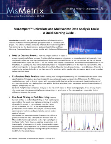
Histograms ask the reader to infer the long term expectation of a variable[Wikipedia]
Histograms summarize variation in a measured variableShows number of samples that occur in a category: called a frequency distribution
Histograms for a continuous variable use category bins (usually of equalsize)We are overfilling to achieve the 1 kg spec. If we can reduce variation: boss gives us araise!
Plot your expectation of these histograms:Irepeated lab measurement to measureg (9.81 m/s2 )Ithis class’s grades for a really easy testIannual income for people in CanadaIbacterial count [number per cubic inch] from deli meat samples
Histograms are all about inferring long-term probabilitiesYou implicitly used a “long” time scale for your prior histogramsOther examples:INext throw on a die? A fair die has a 16.67% chance of showing each number.IWhat is the batch yield tomorrow? Long term average 160 g.L 1 20 g.L 1IBoy or a girl? Canada’s sex ratio at birth 1.06:1 (boy:girl)Age at death? Canadian life tables: e.g. in 2002, for females:IIIhave a 98.86% chance of reaching age 30have a 77.5% chance of reaching age 75
Frequency distributionSee the printed notes for detailed steps to construct a frequency distribution.ICategorical variablesIContinuous variable: with and without quantizationMain steps are:1. Decide what you are measuring2. Resolution for the measurement (x) axis3. Find number of observations in each bin4. Plot it as a bar plot.If you divide bin count by N , then you are plotting the relative frequency.
Data from a reactor: production yield, measured in g/L
Data from a reactor: production yield, measured in g/L
Frequency distribution: you can also use a relative frequencyRelative frequencyI does not require knowing NI can be compared to other distributions (e.g. side-by-side)I for large N it quickly resembles the population’s distributionI area under histogram is equal to 1 (related to probability)
Unpaid housework in two cities: fair comparison are harder with frequencydata alone
Unpaid housework in two cities: fair comparison are harder with frequencydata alone
Unpaid housework in two cities: easier comparison with relative frequencydata
Income of people in Ontario, 2008Rotated here for better reading
Histogram creation in R is very straightforward
We introduce many concepts in this module; many of which you knowalready
Review of terminology you are already comfortable withPopulationLarge collection of potential measurements (not necessary to be infinite, a large Nworks well)SampleCollection of observations that have actually occurred (n samples)In engineering: usually have plenty of data; that often is our population.
Quick review of basic terminologyProbabilityArea under relative frequency distribution curve equals 1.Probability is the fraction of the area under the curve.Construct histograms for yourself, then mark the area:IProbability of grades less than 80%IProbability that number on dice is 1 or 2IBacterial count per cubic inch is above 10,000
Use of the area under a relative frequency histogramProbability
Use of the area under a relative frequency histogramProbability
Quick review of basic terminologyParameterIValue that describes the population’s distribution (fixed)StatisticIAn estimate of one of the population’s parameters (estimate implies that it varies)MeanIMeasure of location (position)E {x} µ 1 XxNSample mean: x̄ 1XxinPopulation mean:ni 1IMean by itself is not sufficient to describe a (random) variable
Quick review of basic terminologyVariance (spread)IMeasure of spread, or variability V {x} E (x µ)2Population variance:IThe population standard deviation σISample variance: s2 IThe sample standard deviation sI σ21 X(x µ)2 Nn1 X(xi x̄)2n 1i 1Degrees of freedom: the denominator term, n 1
Quick review of basic terminologyOutlierA point that is unusual, given the context of the surrounding dataI4024, 5152, 2314, 6360, 4915, 9552, 2415, 6402, 6261I4, 61, 12, 64, 4024, 52, -8, 67, 104, 24Let’s look at the sample statistics:IRegular:x̄ 440.4IRobust: Median 56.5s 1260MAD 57
Outliers are not only univariate; we also have multivariate outliers
Quick review of basic terminologyMedian (location)IOne alternative measure of central tendency.IRobust statistic: insensitive (robust) to outliers in the dataIThe mean is extremely sensitive to outliersThe most robust estimator of sample location:IIIbreakdown of 50%: implies 50% of the data contaminated before median breaksdownbreakdown of the mean is 1/n%: only 1 outlier requiredWhy should you care?Always use the median and MAD (described next) where possible.
Median absolute deviation, MAD (spread)IA robust measure of spreadmad {xi } c · median {kxi median {xi } k}IThe constant c 1.4826 makes MAD consistent with the standard deviation if xiare normally distributed.IBreakdown of MAD: 50%IBreakdown of standard deviation: 1/n%IRead the paper by RousseeuwII(especially 600-level and graduate students):http://yint.org/robust-tutorialAnother robust estimate of spread is the IQR (inter-quartile range), but not asrobust as the MAD
We will take a look at some basic distributions nextIJust a review; please read any of the books listed on the website for more detailsIFocus on when to use the distributionIAnd how the distribution looks
The binary (Bernoulli distribution)For binary events: event A and event BIPass/fail, or yes/no systemIp(pass) p(fail) 1IExample: what is probability ofseeing this sequence ifp(pass) 0.7pass, pass, passIIII(0.7)(0.7)(0.7) 0.343only if each “pass” or “fail” isindependent of the othersamplespass, fail, pass, fail, pass, failI(0.7)(0.3)(0.7)(0.3)(0.7)(0.3)
The uniform distributionEach outcome is equally as likely to occur as all the others. The classic example isdice: each face is equally as likely.Probability distribution for an event with 4 possible outcomes:
Introduction to the normal distributionWe need to look at two topics first:1. The Central Limit Theorem2. The concept of Independence
Central limit theorem, and the important assumptions that go with itCentral limit theoremThe average of a sequence of independent values from any distribution will approximatethe normal distribution, provided the original distribution has finite variance.Assumption: the samples used to compute the average are independent.How is this theorem relevant with engineering data?IIn many cases we are using averages from our raw dataIThese raw data are almost never normally distributedIBut using the assumption that these averages are normally distributed is powerful
The assumption of independence is widely usedIt is a condition for the Central Limit Theorem.IndependenceThe samples are randomly taken from a population. If two samples are independent,there is no possible relationship between any two samples.We frequently violate this assumption in engineering work.Discuss these examples:IThe snowfall, recorded in millimetres, every 6 hours, for 1 week.ISnowfall, recorded on 15 January for every year since 1976: independent or not?IA questionnaire is given to students. Are the answers independent if studentsdiscuss the questionnaire prior to handing it in?IThe impurity values in the last 10 batches of product produced.ISee the exercise in the notes about independence (pump failures).
Which one of these series have independent values in time?
Recap of the central limit theorem from the prior video
The basic normal distribution for a standardized variable
The basic normal distribution for a standardized variable
The ammonia dataset: the raw data and the effect of centering the dataThe raw data: xThe mean ammonia concentration isx 36.The raw data after centering: x x
The ammonia dataset: the centered data and the effect of scalingThese are the centered data: x xThe standard deviation s 8.5.Note: the parameter, σ, is unknown.The statistic, s 8.5 is an estimate of σ.These are the data after scaling:x x1 · (x x)ssx xs
The standard form definitionFor parameters:For statistics:z x µσz x xsIThey are both the same structure.IThe units are removed by cancellation.IStandardization allows us to straightforwardly compare 2 variables that havedifferent means and spreads
Two approximate rules you must remember: 70% rule
Two approximate rules you must remember: 95% rule
The standard form definitionz x µσIx N (µ, σ 2 ) do not use the standard deviation, use σ 2Iz N (0.0, 1.0) after standardizationIHeight of Australians h N (180 cm, 36 cm2 )
Integrating the areas under the curve
Statistical tables (graphical)
Statistical tables (tabular form)
Inverse cumulative distribution (graphical and tabular form)Make sure you can use both R (left) or tables (right).
Integrating the areas under the curve between two pointsLeft point
Integrating the areas under the curve between two pointsRight point
Integrating the areas under the curve between two pointsSubtract out the darker overlap region
Integrating the areas under the curve between two pointsLeaving the net result
Two more worked examples to check your knowledge1. Assume x biological activity of a drug, x N (26.9, 9.3)What is the probability of x 30.0?I30 273 139Find the area under the standard normal distribution: z 1ISo the area 84%IFirst create z variable: z
Two more worked examples to check your knowledge2. Assume x yield from batch process:x N (85 g/L, 16 g2 .L 2 )What is the proportion of yield values between 77 and93 g/L?Ix 85Create both z variables: z 16We get z values of 2 and 2IArea from to 2 is 97.73%IArea from to 2 is 2.27%IFind the area between 2 and 2 as 95%I
Checking for normality. Are these samples normally distributed?
Inverse cumulative distribution function (inverse CDF)IICumulative distribution: area underneath the distribution functionInverse cumulative distribution: we know the area, but want to get back to thevalue along the z-axis.
Checking for normality using q-q plotsApproach: comparepropertiesIuse data from thetheoretical distributionIcompare it with actualdata.We will assume we have Nactual observations to check.1. Create N observations that are normally distributed:
Checking for normality using q-q plotsThis software code shows how you would do this in R:N 10index - seq ( 1 , N )#1,2, .10P - ( index 0 . 5 ) / N# 0.05 , 0.15 , . . . 0.95theoretical . quantity - qnorm ( P )# [ 1 ] 1.64 1.04 0.674 0.385 0.126#0.125 0.385 0.6744 1.036 1.64
Checking for normality using q-q plots2. Standardize the actual data points:I subtract the mean, divide by standard deviationI Sort the data from lowest to highestI These points should now match the theoretical points from step 1 if they arenormally distributed. Example:yields - c ( 8 6 . 2 , 8 5 . 7 , 7 1 . 9 , . . . 8 6 . 9 , 7 8 . 4 )mean . yield - mean ( yields )# 80.0sd . yield - sd ( yields )# 8.35yields . z - ( yields mean . yield ) /sd . yield#[ 1 ] 0 . 7 3 4 0 . 6 7 4 0.978 1 . 8 2 . . . 0.140 0 . 8 1 8 0.2yields . z . sorted - sort ( yields . z )#[ 1 ] 1.34 1.04 0.978 0.355 . . . 0 . 7 3 4 0 . 8 1 81.82theoretical . quantity# see p r i o r s l i d e#[ 1 ] 1.64 1.04 0.674 0.385 . . . 0 . 6 7 4 1 . 0 3 61.64
Checking for normality using q-q plots3. Plot theoretical quantities against the actual quantities.IThey should form a 45 degree line if truly from this distribution
Checking for normality using q-q plots1. Usually we unscale the y-axis (the axis with actual data) so we can see theoriginal data values2. The car library: adds 95% confidence bounds that should contain the data points
Checking for normality. Are these samples normally distributed?
Recap of the prior materialz-value for any variable x is defined as: z x meanstandard deviationWe were also able to derive confidence interval bounds in the prior class:x̄ µ cnσ/ nI cn Iσσx̄ cn µ x̄ cn nnILB µ UB
Central limit theorem: extended New: x̄ N µ, σ 2 /n really powerful statementInterpretationRepeated estimates of mean are unbiased (tends towards µ of the distributionsampled from!) and variance of that estimate is decreased by a factor n.
If we have x N µ, σ 2 then we get x̄ N µ, σ 2 /n
Relaxing the requirement to know σOur current approach:x̄ µI z σ/ nI z N µ, σ 2 /nRaw data are from any distribution of finitevariance.Our revised approach:x̄ µI z s/ nIz t (ν n 1)Additionally requires that the raw data arenormally distributed. easy to verify
Summary of our revised process
The t-distribution is heavily used in this course: let’s examine it a bit moreIt has one parameter: z t (ν), where ν n 1 degrees of freedom. Here ν 8.
Relaxing the requirement to know σOur current approach:x̄ µI z σ/ nOur revised approach:x̄ µI z s/ nI z N µ, σ 2 /nIz t (ν n 1)I cn z cnI ct z ctI cn x̄ µ cnσ/ nI ct Iσσx̄ cn µ x̄ cn nnIssx̄ ct µ x̄ ct nnI17.7 µ 22.3I17.1 µ 22.9x̄ µ cts/ n
Reading values from a table of the t-distribution
Example (continued from the prior videos)Large bale of polymer composite: 9 independent samples taken and sent to lab. Thesamples are independent estimates of the bale’s entire (population) viscosity.Ix 23, 19, 17, 18, 24, 26, 21, 14, 18Ix̄ 20.0Is 3.81The z-value is not known (we do not know µ): find critical lower and upper boundsthat will contain 95% of all possible z-values. ct zleq ctWhat would the ct value be for this example?qt(0.975, df 8)
Confidence Intervals: we have to be very comfortable with this conceptExample: a customer is evaluating your product: they want a confidence interval (CI)for the impurity level in your sulphuric acid over the past year.Response: the range from 429ppm to 673ppm contains the true impurity level with95% confidence.This is a compact representation of the impurity level.Alternatively you could have said:Ithe sample mean from the last year of data is 551 ppmIthe sample standard deviation from the last year [can be back-calculated if wewere told n]Ithe last year of data are normally distributedA CI conveys this information equally well, and in a useful manner.
Summary: confidence interval derivation for the case where the variance,σ 2 , is not known ct s x̄ ct nLB x̄ µ s/ nµµ cts x̄ ct n UBsLB x̄ ct nsUB x̄ ct nDo you recall the important assumptions that lead to these results?
Interpreting the confidence interval (CI) incorrectlyIx 23, 19, 17, 18, 24, 26, 21, 14, 18Ix̄ 20.0Is 3.81Ict 2.31 for the 95% confidence interval with 8 degrees of freedomILB 20.0 2.92 17.1IUB 20.0 2.92 22.9IThe CI does not imply that x̄ lies in the interval from LB to UB, i.e. the CI isnot about x̄; it’s about µIIncorrect to say: (sample) average viscosity is 20 units and lies inside the rangeof 17.1 to 22.9 with a 95% probability
Interpreting the confidence interval (CI) correctlyILB 20.0 2.92 17.1IUB 20.0 2.92 22.9IThe CI does imply that µ is expected to lie within that interval, with the givenlevel of confidenceIThe CI is a range of possible values for µ, not for x̄.IUB and LB are a function of the data sampleIf we take a different sample of data, we will get different boundsIIIIIIf confidence level is 95%, then 5% of the time the interval will not contain the truemeanCollect 20 sets of samples, 19 times out of 20 the CI range will contain the true meanIT IS NOT: Probability that the true population viscosity, µ is within the givenrange [µ doesn’t have a probability; it is 100% fixed]IT IS: Probability that the CI range contains the true population viscosity, µ
Interpreting the confidence interval by altering the sample, process, orconfidence levelsx̄ ct ns µ x̄ ct nIAs n increases, the confidence interval range decreasesbut with diminishing returns (intuitively expected)IWe could have adjusted s as well.IWe can arbitrarily select our level of confidence:IConfidence level90%95%99%ILB17.617.115.7What happens if the level of confidence is 100%?IThe confidence interval is then infinite.UB22.422.924.2
Summary: confidence for interval for the parameter µ, the meanMake an assumption about the raw data:In independent points this assumption is always requiredWe know the population σz We do not know the population σx̄ µ σ/ nz x̄ µ s/ nIAlso, we require x N (µ, σ 2 /n)Ix̄ N (µ, σ 2 /n)Ix̄ t(ν n 1)Iσσx̄ cn µ x̄ cn nnIssx̄ ct µ x̄ ct nnIqnorm(0.975) when at the 95%confidence levelIqt(0.975, df .) when at the95% confidence level
Comparison between the two cases: how does it matter?You can prove the confidence interval with unknown variance is wider. (600-levelstudents . why?) We expect this intuitively:Iit reflects our uncertainty of the spread parameter: s vs σIleads to a more conservative result (i.e. wider bound)
Many other confidence intervals existIThey exist for population variances: LB σ 2 UBIIratio of two variances: do these 2 samples have same variance?They exist for proportions:IIproportion of packaged pizzas with N or more pepperoni slices is between 86 and92%political polls: party XYZ has 35% of the vote, the margin of error is 3%; accurate19 times out of 20
A worked exampleYour manager is asking for the average viscosity of a product that you produce in abatch process.Recorded below are the 12 most recentvalues, taken from consecutive batches.State any assumptions, and clearly showthe calculations which are required toestimate a 95% confidence interval for themean.Interpret that confidence interval for yourmanager, who is not sure what aconfidence interval is.13.7, 14.9, 15.7, 16.1, 14.7, 15.2,13.9, 13.9, 15.0, 13.0, 16.7, 13.2[Flickr: 2516220152]
A worked example: what assumptions are being made?IWe can assume the sample average x̄ NIWe don’t know σ; so we must estimate it.x̄ µThat means z t(ν)s/ nwhich in turn requires us to assume the raw data, xi NII
A worked example: lets do the calculations and interpret the resultIssx̄ ct µ x̄ ct nns 1.16Ict 2.2I14.67 II2.2 1.162.20 1.16 µ 14.67 121213.9 µ 15.4IInterpretation: the range has a 95% probability of containing the true viscosity.
A worked example: a cautionWe also need to clean the batch reactorproperly between every use.There are other ways that independencecan be violated: what about raw materiallots and operators running the batch?In practice, we will definitely violate thisassumption to some extent.[Flickr: 2516220152]
The batch yield feedback case studyYour manager is asking for the average viscosity of a product that you produce in abatch process.IMost recent 10 batches run, using theexisting system (A): average yield isx̄A 79.9%IPut on a prototype control system (B)and run 10 batches: x̄B 82.9%Ix̄B x̄A 82.93 79.89 3.04%IWas this just lucky, or is this apermanent improvement? What’s therisk we are wrong?[Flickr: 2516220152]
Let’s look at the raw data: table form
Let’s look at the raw data: box plot of the data
Let’s look at the raw data: given the context of prior batches
One approach: compare the data to a reference set1. We have 300 previous batches operating with system AIICalculate average from batch 1, 2, 3, . 10Calculate average from batch 11, 12, 13, . 202. Subtract averages: (group average 11 to 20) minus (group average 1 to 10)3. Shift and repeat steps 2 and 3: use batches (2 to 11) and (12 to 21)4. Collect all the difference values
The question we want to answerLet’s assume the new system B is no different.We assume that 3% increase was pure luck.How many times, in the past, did we observe 3% improvements between two sets of 10consecutive batches?If our assumption at the top of the slide is correct, we should not see many 3%improvements.
A good visualization tool: the dot plotI31 historical differences out of 281 had a difference value higher than 3.04I11% of historical batches had a better difference, by chance, not due to thefeedback controller change.No assumption of independence, nor any form of distribution assumed!Advanced students: plot a time-series plot of these data, for an even greater insight towhat is occurring here.
Has a significant change occurred in the system?Our key focus this time: we have limited data. We say,“there is no external reference set available”.In the prior example, we have plenty of historical data:
Second approach: when no reference data is availableIDon’t have a suitable reference, e.g. just the 20 runsIWe will take a look at the method, and assumptionsAim: is µB µA ? In other words, is µB µA 0?21. Assume data for case A is normally distributed: A N µA , σA 22. Assume data for case B is normally distributed: B N µB , σB 3. Assume data for sample A and sample B have σA σB σ4. From CLT (assumes data in A and data in B are independent)II2σAnAσ2V {x̄B } BnBV {x̄A }
Second approach: when no reference data is available5. Assume: x̄A and x̄B are independent [likely true in many cases] σ211σ22I V {x̄B x̄A } σ nA n BnA nB6. Create a z-value:Iz (variable “x”) (“location”)(x̄B x̄A ) (µB µA )s “spread”112σ nA nB7. Create a confidence interval for zr r 112(x̄B x̄A ) cn σ nA nB µB µA (x̄B x̄A ) cn σ 2 n1A 1nB
Back to method 2 for testing differencesAim: is µB µA ? In other words, is µB µA 0?1. Assume sample A2. Assume equal variance: σA σB σ3. So from CLT:σ2σ2I V {x̄A } A and V {x̄B } BnAnB4. Assume: x̄A and x̄B are independent - so combine variances: σ211σ22I V {x̄B x̄A } σ nA n BnA nB6. Create z-value. Ask: what is our probability/risk?(x̄B x̄A ) (µB µA )I z s 112σ nA nB
Method 2b: No reference set, internal σIIIs2Ps2PSample variances: s2A 6.812 and s2B 6.702It just happens that nA nB 10 (can have nA 6 nB )Pool (combine) the variance, using a weighted sum:(nA 1)s2A (nB 1)s2B nA 1 nB 1 z z 9 6.812 9 6.702 45.6318(x̄B x̄A ) (µB µA )s 112sP 10 103.04 0p 1.0145.63 2/10Probability of z 1.01? The area from up to 1.01 is 83.7% using the t
titler (x̄B x̄A ) ct s2P n1A 1nB r µB µA (x̄B x̄A ) cts2P 1nA 1nB
Example of testing for differences: impellersTry these cases:I43 min µAxial µRadial 95 minI 95 min µRadial µAxial 43 minI 12 min µAxial µRadial 7 minI 453 min µAxial µRadial 284 minI 21 min µAxial µRadial 187 minWhat is your recommendation for choosing the one impeller over the other?Consider the case of statistical difference vs engineering difference
General principle when testing for significant differencesKeep everything as constant as possible, except the feature under investigationIn the section on “Designed Experiments” we will vary more than 1 item.[Flickr: 2516220152]
The key equation derived in the prior videos on confidence intervalsr(x̄B x̄A ) cts2P 1nA 1nB µ B µAr (x̄B x̄A ) ct s2P n1A lower bound µB µA upper boundsP , the pooled standard deviation1nB
4 000 L reactor[Image credits: Wikipedia (left) and Flickr: 13193170764 (right)]Raw material size: 8 000 L
For paired testing: always be clear on your goalIn this example: what is the effect on conversion, either with baffles or without baffles?Our hope for this test (these data are guesses; we have not done the work yet)Without baffles [4 000 L]With baffles [4 000 L]Difference in results2. conversion: 72%1. conversion: 78%Batch 1 2:6%4. conversion: 74%3. conversion: 78%Batch 3 4:4%6. conversion: 70%5. conversion: 75%Batch 5 6:5%We are going to analyze our actual data like this, later on.
Why should we go to all this trouble of setting up the experiments?The effect of raw materials is consistent; we want to cancel it out.Assume the raw materials have an effect of h; we will use a value of h 3% here.Without bafflesWith bafflesITrue conversion 71%ITrue conversion 75%IBias of h 3%IBias of h 3%IConversion recorded 74%IConversion recorded 78%A common, constant source of variation is removed,and we don’t need to know the constant!Difference in resultsI78 74 4%(75 h) (71 h)75 71 h h 4%
When should you use a paired test?A paired test is appropriate when there is something in common within pairs ofsamples in group A and B.But the commonality is not between the pairs.In our example:Iwithin-pair commonality is the raw material
How not to run paired experiments1. Sequentially assign A and B (don’t ever do this!)A A A A A B B B B B1 1 2 2 3 3 4 4 5 5IThis will certainly lead to confounding with an unintentional factor2. Randomly assign A and B (commonality between pairs won’t cancel)A A B B B A A B A B1 1 2 2 3 3 4 4 5 5
Paired tests: so how do I analyze data from such a test?1. Calculate the differences: w [w1 , w2 , . . . , wn ]IIIIIThere ar
References and readings I Any standard statistics text book I Recommended: Box, Hunter and Hunter, Statistics for Experimenters, Chapter 2 (both 1st and 2nd edition) I Wikipedia articles on any term that seems unfamiliar or that you've forgotten I Hodges and Lehmann, Basic Concepts of Probability and Statistics I Hogg and Ledolter, Engineering Statistics I Montgomery and Runger, Applied .