WIXLIB

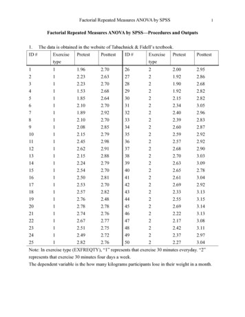
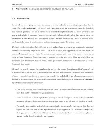
CHAPTER 5ST 732, M. DAVIDIANThis assumption might be reasonable for the upper two units in panel (b), as the “inherenttrends” for these units are roughly parallel to the trajectory of means over time. But the lowerunit’s trend is far below the mean at early times but rises to be above it at later times; for thisunit, the deviation from the mean is not the same at all times.As we will see shortly, violation of this assumption may not be critical as long as the overallpattern of variance and correlation implied by this model is similar to that in the data.Figure 2: (a) Hypothetical longitudinal data from m 3 units at n 9 time points. (b) Conceptualrepresentation of sources of variation.(a)(b)PSfrag replacementsµρ12 0.0responseσ22responseσ12ρ12 0.8y1y2timetimeNORMALITY AND VARIANCE ASSUMPTIONS: For continuous responses like those in the example,it is often realistic to consider the normal distribution as a model for the way in which the varioussources of variation affect the response. If Yh j is continuous, we would expect that the deviations dueto biological variation (among-units) and within-unit sources that affect how Y h j turns out to also becontinuous. Thus, rather than assuming that Yh j is normally distributed directly, it is customary toassume that each random component arises from a normal distribution.Specifically, the standard assumptions, which also incorporate assumptions about variance, are: bh N (0, σb2 ) and are all independent. This says that the distribution of deviations in the population of units is centered about 0 (some are negative, some positive), with variation characterizedby the variance component σb2 .PAGE 111

CHAPTER 5ST 732, M. DAVIDIANThe fact that this normal distribution is identical for all 1, . . . , q reflects an assumptionthat units vary similarly among themselves in all q populations. The independence assumptionrepresents the reasonable view that the response one unit in the population gives at any time iscompletely unrelated to that given by another unit. eh j N (0, σe2 ) and are all independent. This says that the distribution of deviations due towithin-unit causes is centered about 0 (some negative, some positive), with variation characterized by the (common) variance component σe2 .That this distribution is the same for all 1, . . . , q and j 1, . . . , n again is an assumption.The variance σe2 represents the “aggregate” variance of the combined fluctuation and measurementerror processes, and is assumed to be constant over time and group. Thus, the model assumesthat the combined effect of within-unit sources of variation is the same at any time in all groups.E.g. the magnitude of within-unit fluctuations is similar across groups and does not change withtime, and the variability associated with errors in measurement is the same regardless of the sizeof the thing being measured.The independence assumption is something we must think about carefully. It is customary toassume that the error in measurement introduced by, say, an imperfect scale at one time pointis not related to the error in measurement that occurs at a later time point; i.e. measurementerrors occur “haphazardly.” Thus, if eh j represents mostly measurement error, the independenceassumption seems reasonable. However, fluctuations within a unit may well be correlated, asdiscussed in the last chapter. Thus, if the time points are close enough together so that correlationsare not negligible, this may not be reasonable. (recall our discussion of observations close in timetending to be “large” or “small” together). The bh and eh j are assumed to all be mutually independent. This represents the view thatdeviations due to within-unit sources are of similar magnitude regardless of the the magnitudesof the deviations bh associated with the units on which the observations are made. This is oftenreasonable; however, as we will see later in the course, there are certain situations where it maynot be reasonable.With these assumptions it will follow that the Yh j s are normally distributed, as we will now demonstrate.VECTOR REPRESENTATION AND COVARIANCE MATRIX: Now consider the data on a particularunit. With this notation, the subscripts h and identify a particular unit as the hth unit in the thgroup.PAGE 112

CHAPTER 5ST 732, M. DAVIDIANFor this unit, we may summarize the observations at the n times in a vector and write Yh 1 Yh 2 . . . Yh n µ τ γ1 (τ γ) 1 µ τ γ2 (τ γ) 2 . . µ τ γn (τ γ) n bh bh . . . bh eh 1 eh 2 . . . eh n (5.3)Y h µ 1bh eh ,where 1 is a (n 1) vector of 1s, or more succinctly, Yh 1 Yh 2 . . . Yh n µ 1 µ 2 . . . µ n ²h 1 ²h 2 . . . ²h n (5.4)Y h µ ²h ,so, for the data vector from the hth unit in group ,E(Y h ) µ .We see that the model implies a very specific representation of a data vector. Note that for all unitsfrom the same group ( ) µ is the same.We will now see that the model implies something very specific about how observations within andacross units covary and about the structure of the mean of a data vector. Because bh and eh j are independent, we havevar(Yh j ) var(bh ) var(eh j ) 2cov(bh , eh j ) σb2 σe2 0 σb2 σe2 . Furthermore, because each random component bh and eh j is normally distributed, each Yh j isnormally distributed. In fact, the Yh j values making up the vector Y h are jointly normally distributed.Thus, a data vector Y h under the assumptions of this model has a multivariate (n-dimensional) normaldistribution with mean vector µ . We now turn to the form of the covariance matrix of Y h .PAGE 113

CHAPTER 5ST 732, M. DAVIDIANFACT: First we note the following result. If b and e are two random variables with means µ b and µe ,then cov(b, e) 0 implies that E(be) E(b)E(e) µb µe . This is shown as follows:cov(b, e) E(b µb )(e µe ) E(be) E(b)µe µb E(e) µb µe E(be) µb µe .Thus, cov(b, e) 0 E(be) µb µe , and the result follows. We know that if b and e are jointly normally distributed and independent, then cov(b, e) 0. Thus, b and e independent and normal implies E(be) µb µe . If furthermore b and e have means0, i.e. E(b) 0, E(e) 0, then in factE(be) 0.We now use this result to examine the covariances. First, let Yh j and Yh0 0 j 0 be two observations taken from different units (h and h0 ) from differentgroups ( and 0 ) at different times (j and j 0 ).cov(Yh j , Yh0 0 j 0 ) E(Yh j µ j )(Yh0 0 j 0 µ 0 j 0 ) E(bh eh j )(bh0 0 eh0 0 j 0 ) E(bh bh0 0 ) E(eh j bh0 0 ) E(bh eh0 0 j 0 ) E(eh j eh0 0 j 0 )(5.5)Note that, since all the random components are assumed to be mutually independent with 0means, by the above result, we have that each term in (5.5) is equal to 0! Thus, (5.5) implies thattwo responses from different units in different groups at different times are not correlated. In fact, the same argument goes through if 0 , i.e. the observations are from two differentunits in the same group and/or j j 0 , i.e. the observations are from two different units at thesame time. That is (try it!),cov(Yh j , Yh0 j 0 ) 0, cov(Yh j , Yh0 0 j ) 0, cov(Yh j , Yh0 j ) 0. Thus, we may conclude that the model (5.1) automatically implies that any two observationsfrom different units have 0 covariance. Furthermore, because these observations are all normallydistributed, this implies that any two observations from different units are independent! Thus,two vectors Y h and Y h0 0 from different units, where 6 0 or 0 , are independent underthis model!Recall that at the end of Chapter 3, we noted that it seems reasonable to assume that data vectorsfrom different units are indeed independent; this model automatically induces this assumption.PAGE 114

CHAPTER 5ST 732, M. DAVIDIAN Now consider 2 observations on the same unit, say the hth unit in group , Y h j and Yh j 0 . Wehavecov(Yh j , Yh j 0 ) E(Yh j µ j )(Yh j 0 µ j 0 ) E(bh eh j )(bh eh j 0 ) E(bh bh ) E(eh j bh ) E(bh eh j 0 ) E(eh j eh j 0 ) σb2 0 0 0 σb2 .(5.6)This follows because all of the random variables in the last three terms are mutually independentaccording to the assumptions andE(bh bh ) E(bh 0)2 var(bh ) σb2by the assumptions.COVARIANCE MATRIX: Summarizing this information in the form of a covariance matrix, we seethat var(Y h ) σb2 σe2σb2.σb2σb2σb2 .σe2σb2······.σb2σb2.· · · σb2 σe2 (5.7) Actually, we could have obtained this matrix more directly by using matrix operations applied tothe matrix form of (5.3). Specifically, because bh and the elements of eh are independent andnormal, 1bh and eh are independent, multivariate normal random vectors,var(Y h ) var(1bh ) var(eh ) 1var(bh )10 var(eh ).(5.8)Now var(bh ) σb2 . Furthermore (try it), 011 J n 1 ··· 1 1 ··· 1 1 ··· 1 and var(eh ) σe2 I n ;. . . . . . applying these to (5.8) givesvar(Y h ) σb2 J n σe2 I n Σ.(5.9)It is straightforward to observe by writing out (5.9) in detail that it is just a compact way, inmatrix notation, to state (5.7).PAGE 115

CHAPTER 5ST 732, M. DAVIDIAN It is customary to use J to denote a square matrix of all 1s, where we add the subscript when wewish to emphasize the dimension. We thus see that we may summarize the assumptions of model (5.1) in matrix form: The m datavectors Y h , h 1, . . . , r , 1, . . . , q are all independent and multivariate normal withY h Nn (µ , Σ),where Σ is given in (5.9).COMPOUND SYMMETRY: We thus see from given in (5.7) and (5.9) is that this model assumes thatthe covariance of a random data vector has the compound symmetry or exchangeable correlationstructure (see Chapter 4). Note that the off-diagonal elements of this matrix (the covariances among elements of Y h ) areequal to σb2 . Thus, if we compute the correlations, they are all the same and equal to (verify)σb2 /(σb2 σe2 ). This is called the intra-class correlation in some contexts. As we noted earlier, this model says that no matter how far apart or near in time two elementsof Y h were taken, the degree of association between them is the same. Hence, with respect toassociation, they are essentially interchangeable (or exchangeable). Moreover, the association is positive; i.e. because both σb2 and σe2 are variances, both arepositive. Thus, the correlation, which depends on these two positive quantities, must also bepositive. The diagonal elements of are also all the same, implying that the variance of each element of Y h is the same. This covariance structure is a special case of something called a Type H covariance structure.More on this later. As we have noted previously, the compound symmetric structure may be a rather restrictiveassumption for longitudinal data, as it tends to emphasize among-unit sources of variation. Ifthe within-unit source of correlation (due to fluctuations) is non-negligible, this may be a poorrepresentation. Thus, assuming the model (5.1) implies this fairly restrictive assumption on thenature of variation within a data vector.PAGE 116

CHAPTER 5ST 732, M. DAVIDIAN The implied covariance matrix (5.7) is the same for all units, regardless of group.As we mentioned earlier, using model (5.1) as the basis for analyzing longitudinal data is quite commonbut may be inappropriate. We now see why – the model implies a restrictive and possibly unrealisticassumption about correlation among observations on the same unit over time!ALTERNATIVE NOTATION: We may in fact write the model in our previous notation. Note that hindexes units within groups, and indexes groups, for a total of m Pq 1 r units. We could thusreindex units by a single index, i 1, . . . , m, where the value of i for any given unit is determined byits (unique) values of h and . We could reindex bh and eh in the same way. Thus, let Y i , i 1, . . . , m,i.e. Yi Yi1.Yin , denote the vectors Y h , h 1, . . . , r , 1, . . . , q reindexed, and similarly write bi and ei . To expressthe model with this indexing, the information on group membership must somehow be incorporatedseparately, as it is no longer explicit from the indexing. To do this, it is common to write the model asfollows.Let M denote the matrix of all means µ j implied by the model (5.1), i.e. M µ11 µ12 · · · µ1n.µq1 µq2 · · · µqn . The th row of the matrix M in (5.10) is thus the transpose of the mean vector µ (n 1), i.e. M µ01.µ0qPAGE 117 . (5.10)

CHAPTER 5ST 732, M. DAVIDIANAlso, using the new indexing system, let, for 1, . . . , q,ai 1 if unit i is from group 0 otherwiseThus, the ai record the information on group membership. Now let ai be the vector (q 1) of ai values corresponding to the ith unit, i.e.a0i (ai1 , ai2 , . . . , aiq );because any unit may only belong to one group, ai will be a vector of all 0s except for a 1 in the positioncorresponding to i’s group. For example, if there are q 3 groups and n 4 times, then µ11 µ12 µ13 µ14 M µ21 µ22 µ23 µ24 µ31 µ32 µ33 µ34 and if the ith unit is from group 2, thena0i (0, 1, 0),so that (verify)a0i M (µ21 , µ22 , µ23 , µ24 ) µ0i ,say, the mean vector for the ith unit. The particular elements of µi are determined by the groupmembership of unit i, and are the same for all units in the same group.Using these definitions, it is straightforward (try it) to verify that we may rewrite the model in (5.3)and (5.4) asY 0i a0i M 10 bi e0i , i 1, . . . , m.andY 0i a0i M ²0i , i 1, . . . , m.(5.11)This one standard way of writing the model when indexing units is done with a single subscript (i inthis case).In particular, this way of writing the model is used in the documentation for SAS PROC GLM. Theconvention is to put the model “on its side,” which can be confusing.PAGE 118

CHAPTER 5ST 732, M. DAVIDIANAnother way of writing the model that is more familiar and more germane to our later development isas follows. Let β be the vector of all parameters in the model (5.1) for all groups and times; i.e. all ofµ, the τ , γj , and (τ γ) j , 1, . . . , q, j 1, . . . , n. For example, with q 2 groups and n 3 timepoints, β µτ1τ2γ1γ2γ3(τ γ)11(τ γ)12(τ γ)13(τ γ)21(τ γ)22(τ γ)23Now E(Y i ) µi . If, for example, i is in group 2, then . µ21 µ τ2 γ1 (τ γ)21 µi µ22 µ τ2 γ2 (τ γ)22 Note that if we defineµ23µ τ2 γ3 (τ γ)23 . 1 0 1 1 0 0 0 0 0 1 0 0 Xi 1 0 1 0 1 0 0 0 0 0 1 0 ,then (verify), we can write 1 0 1 0 0 1 0 0 0 0 0 1 µi X i β.Thus, in any general model, we see that, if we define β and X i appropriately, we can write the modelasY i X i β 1bi eior Y i X i β ²i , i 1, . . . , m.X i would be the appropriate matrix of 0s and 1s, and would be the same for each i in the same group.PAGE 119

CHAPTER 5ST 732, M. DAVIDIANPARAMETERIZATION: Just as with any model of this type, we note that representing the means µ jin terms of parameters µ, τ , γj , and (τ γ) j leads to a model that is overparameterized. That is,while we do have enough information to figure out how the means µ j differ, we do not have enoughinformation to figure out how they break down into all of these components. For example, if we had 2treatment groups, we can’t tell where all of µ, τ1 , and τ2 ought to be just from the information at hand.To see what we mean, suppose we knew that µ τ1 20 and µ τ2 10. Then one way this couldhappen is ifµ 15, , τ1 5, τ2 5;another way isµ 12, , τ1 8, τ2 2;in fact, we could write zillions of more ways. Equivalently, this issue may also be seen by realizing thatthe matrix X i is not of full rank.Thus, the point is that, although this type of representation of a mean µ j used in the context of analysisof variance is convenient for helping us think about effects of different factors as deviations from an“overall” mean, we can’t identify all of these components. In order to identify them, it is customary toimpose constraints that make the representation unique by forcing only one of the possible zillions ofways to hold:qX 1τ 0,nXj 1γj 0,qX(τ γ) j 0 1nX(τ γ) j for all j, .j 1Imposing these constraints is equivalent to redefining the vector of parameters β and the matrices X iso that X i will always be a full rank matrix for all i.REGRESSION INTERPRETATION: The interesting feature of this representation is that it looks likewe have a set of m “regression” models, indexed by i, each with its own “design matrix” X i and“deviations” ²i . We will see later that more flexible models for repeated measurements are also of thisform; thus, writing (5.1) this way will allow us to compare different models and methods directly.Regardless of how we write the model, it is important to remember that an important assumption ofthe model is that all data vectors are multivariate normal with the same covariance matrix having avery specific form; i.e. with this indexing, we haveY i Nn (µi , Σ), Σ σb2 J n σe2 I n .PAGE 120

CHAPTER 55.3ST 732, M. DAVIDIANQuestions of interest and statistical hypothesesWe now focus on how questions of scientific interest may be addressed in the context of such a modelfor longitudinal data. Recall that we may write the model as in (5.11), i.e.Y 0i a0i M ²0i , i 1, . . . , m,where M andµ11 µ12 · · · µ1n.µq1 µq2 · · · µqn(5.12) µ j µ τ γj (τ γ) j .The constraintsqX 1τ 0,nXγj 0,j 1qX(τ γ) j 0 1(5.13)nX(τ γ) jj 1are assumed to hold.The model (5.12) is sometimes written succinctly asY AM ²,(5.14)where Y is the (m n) matrix with ith row Y 0i and similarly for ², and A is the (m q) matrix withith row a0i . We will not make direct use of this way of writing the model; we point it out as it is theway th

5 Univariate repeated measures analysis of variance 5.1 Introduction As we will see as we progress, there are a number of approaches for representing longitudinal data in terms of a statistical model. Associated with these approaches are appropriate methods of analysis that focus on questions that are of interest in the context of longitudinal .