Transcription
1Logistic Regression: Univariate andMultivariate
2Events and Logistic RegressionILogisitic regression is used for modelling eventprobabilities.IExample of an event: Mrs. Smith had a myocardialinfarction between 1/1/2000 and 31/12/2009.IThe occurrence of an event is a binary (dichotomous)variable. There are two possibilities: the event occurs or itdoes not occur.IFor this reason, event occurrence variables can always becoded with 0, 1 e.g.Yi 1 person i became pregnant in 2011.Yi 0 person i did not become pregnant in 2011.
3Measuring the Probability of an EventIThere are many equivalent ways of measuring theprobability of an event.IWe will use three:I1probability of the event2odds in favour of the event3log-odds in favour of the eventThese are equivalent in the sense that if you know thevalue of one measure for an event you can compute thevalue of the other two measures for the same eventcf. measuring a distance in kilometres, statute miles ornautical miles
The Probability of an EventIThis is a number π between 0 and 1. We writeπ P(Y 1)to mean π is the probability that Y 1.Iπ 1 means we know the event is certain to occur.Iπ 0 means we know the event is certain not to occur.IValues between 0 and 1 represent intermediate states ofcertainty, ordered monotonically.IBecause we are certain one of Y 1 and Y 0 is true andbecause they cannot be true simultaneously:P(Y 0) 1 P(Y 1) 1 π.4
5Odds in Favour of an EventIThe odds in favour of an event is defined as theprobability the event occurs divided by the probability theevent does not occur.IThe odds in favour of Y 1 is defined as:ODDS(Y 1) IP(Y 1)πP(Y 1) .P(Y 6 1)P(Y 0)1 πNote:ODDS(Y 0) 11 π .ODDS(Y 1)πsoODDS(Y 1) ODDS(Y 0) 1.
6Interpreting the Odds in Favour of an EventIAn odds is a number between 0 and .IAn odds of 0 means we are certain the event does notoccur.IAn increased odds corresponds to increased belief in theoccurrence of the event.IAn odds of 1 corresponds to a probability of 1/2.IAn odds of corresponds to certainty the event occurs.
7Log-odds in Favour of an EventIThe log odds in favour of an event is defined as the log ofthe odds in favour of the event:log ODDS(Y 1) logIπP(Y 1) log.P(Y 0)1 πNotelog ODDS(Y 1) log ODDS(Y 0) log1 ππ
8Interpreting the Log-odds in Favour of an EventIA log-odds is a number between and .IA log odds of means we are certain the event doesnot occur.IAn increased log-odds corresponds to increased belief inthe occurrence of the event.IA log-odds of 0 corresponds to a probability of 1/2.IA log-odds of corresponds to certainty the event occurs.
9Moving between Probability, Odds and Log-oddsIYou can use the following table to compute one measureof probability from another:PP(Y 1) πODDS(Y 1) olog ODDS(Y 1) xODDSlog ODDSπ1 ππlog 1 πo1 oex1 exlog oexIChoose the row corresponding to the quantity you startwith and the column corresponding to the quantity youwant to compute.Iπlog 1 πis often written logit(π).Iexp(x)1 exp(x)is often written inv. logit(x) (sometimes expit(x)).
Motivation for (Multivariate) Logistic RegressionIWe want to model P(Y 1) in terms of a set of predictorvariables X1 , X2 ,. Xp (for univariate regression p 1).IIn linear regression we use the regression equationE(Y) β0 β1 X1 β2 X2 . βp XpIHowever, for a binary Y (0 or 1), E(Y) P(Y 1).IWe cannot now use equation (?), because the left handside is a number between 0 and 1 while the right handside is potentially a number between and .ISolution: replace the LHS with logit EY :logit E(Y) β0 β1 X1 β2 X2 . βp Xp10(1)
Logistic Regression Equation Written on Three ScalesIWe defined the regression equation on the logit orlog ODDS scale:log ODDS(Y 1) β0 β1 X1 β2 X2 . βp XpIOn the ODDS scale the same equation may be written:ODDS(Y 1) exp(β0 β1 X1 β2 X2 . βp Xp )IOn the probability scale the equation may be written:P(Y 1) 11exp(β0 β1 X1 β2 X2 . βp Xp )1 exp(β0 β1 X1 β2 X2 . βp Xp )
Interpreting the InterceptIIn order to obtain a simple interpretation of the interceptwe need to find a situation in which the other parameters(β1 , ., βp ) vanish.IThis happens when X1 , X2 ., Xp are all equal to 0.IConsequently we can interpret β0 in 3 equivalent ways:I121β0 is the log-odds in favour of Y 1 whenX1 X2 . Xp 0.2β0 is such that exp(β0 ) is the odds in favour of Y 1 whenX1 X2 . Xp 0.30β0 is such that 1 exp(βis the probability that Y 1 when0)X1 X2 . Xp 0.exp(β )You can choose any one of these three interpretationswhen you make a report.
13Pr(Y 1) inv. logit(β0 β1 X1 )Univariate Picture: Intercept10.80.6exp(β0 )1 exp(β0 )0.40.20 2 10123X1IP(Y 1) vs. X1 when p 1 (univariate regression).
14Univariate Picture: Sign of β1Pr(Y 1)10.50 202X1IWhen β1 0, P(Y 1) increases with X1 (blue curve).IWhen β1 0, P(Y 1) decreases with X1 (red curve).
15Univariate Picture: Magnitude of β1Pr(Y 1)10.50 202X1Iβ1 2 (blue curve), β1 4 (red curve).IWhen β1 is greater, changes in X1 more stronglyinfluence the probability that the event occurs.
Interpreting β1 : Univariate Logistic RegressionITo obtain a simple interpretation of β1 we need to find away to remove β0 from the regression equation.IOn the log-odds scale we have the regression equation:log ODDS(Y 1) β0 β1 X1IThis suggests we could consider looking at the differencein the log odds at different values of X1 , say t z and t.log ODDS(Y 1 X1 t z) log ODDS(Y 1 X1 t)which is equal toβ0 β1 (t z) (β0 β1 t) zβ1 .16
17Interpreting β1 : Univariate Logistic RegressionIBy putting z 1 we arrive at the following interpretationof β1 :β1 is the additive change in the log-odds in favour of Y 1when X1 increases by 1 unit.IWe can write an equivalent second interpretation on theodds scale:exp(β1 ) is the multiplicative change in the odds in favour ofY 1 when X1 increases by 1 unit.
β1 as a Log-odds RatioIThe first interpretation of β1 expresses the equation:logODDS(Y 1 X1 t z) zβ1ODDS(Y 1 X1 t)whilst the second interpretation expresses the equation:ODDS(Y 1 X1 t z) exp(zβ1 ).ODDS(Y 1 X1 t)I181 t z)The quantity ODDS(Y 1 XODDS(Y 1 X1 t) is the odds-ratio in favourof Y 1 for X1 t z vs. X1 t.
19Interpreting Coefficients in Multivariate LogisticRegressionIThe interpretation of regression coefficients inmultivariate logistic regression is similar to theinterpretation in univariate regression.IWe dealt with β0 previously.IIn general the coefficient βk (corresponding to the variableXk ) can be interpreted as follows:βk is the additive change in the log-odds in favour of Y 1when Xk increases by 1 unit, while the other predictor variablesremain unchanged.IAs in the univariate case, an equivalent interpretation canbe made on the odds scale.
20Fitting a Logistic Regression in RIWe fit a logistic regression in R using the glm function: output - glm(sta sex, data icu1.dat, family binomial)IThis fits the regression equationlogit P(sta 1) β0 β1 sex.Idata icu1.dat tells glm the data are stored in the dataframe icu1.dat.Ifamily binomial tells glm to fit a logistic model.IAs an aside, we can use glm as an alternative to lm to fit alinear model, by specifying family gaussian.
21Logistic Regression: glm Output in RCall:glm(formula sta sex, family binomial, data icu1.dat)Deviance Residuals:Min1QMedian-0.6876 -0.6876 -0.65593Q-0.6559Max1.8123Coefficients:Estimate Std. Error z value Pr( z )(Intercept) -1.42710.2273 -6.278 3.42e-10 ***sex10.10540.36170.2910.771--Signif. codes: 0 ’***’ 0.001 ’**’ 0.01 ’*’ 0.05 ’.’ 0.1 ’ ’ 1ISummary of the distribution of the deviance residuals.IDeviance residuals measure how well the observations fitthe model. The closer a residual to 0 the better the fit ofthe observation.
22Logistic Regression: glm Output in RCall:glm(formula sta sex, family binomial, data icu1.dat)Deviance Residuals:Min1QMedian-0.6876 -0.6876 -0.65593Q-0.6559Max1.8123Coefficients:Estimate Std. Error z value Pr( z )(Intercept) -1.42710.2273 -6.278 3.42e-10 ***sex10.10540.36170.2910.771--Signif. codes: 0 ’***’ 0.001 ’**’ 0.01 ’*’ 0.05 ’.’ 0.1 ’ ’ 1IIβ̂0 , the maximum likelihood estimate of the interceptcoefficient β0 .exp(β̂0 )1 exp(β̂0 )is an estimate of P(sta 1) when sex 0
23Logistic Regression: glm Output in RCall:glm(formula sta sex, family binomial, data icu1.dat)Deviance Residuals:Min1QMedian-0.6876 -0.6876 -0.65593Q-0.6559Max1.8123Coefficients:Estimate Std. Error z value Pr( z )(Intercept) -1.42710.2273 -6.278 3.42e-10 ***sex10.10540.36170.2910.771--Signif. codes: 0 ’***’ 0.001 ’**’ 0.01 ’*’ 0.05 ’.’ 0.1 ’ ’ 1ISE(β̂0 ), the standard error of the maximum likelihoodestimate of β0 .
24Logistic Regression: glm Output in RCall:glm(formula sta sex, family binomial, data icu1.dat)Deviance Residuals:Min1QMedian-0.6876 -0.6876 -0.65593Q-0.6559Max1.8123Coefficients:Estimate Std. Error z value Pr( z )(Intercept) -1.42710.2273 -6.278 3.42e-10 ***sex10.10540.36170.2910.771--Signif. codes: 0 ’***’ 0.001 ’**’ 0.01 ’*’ 0.05 ’.’ 0.1 ’ ’ 1Iz-value for a Wald-statistic, z β̂0 /SE(β̂0 )Ip-value for test of null hypothesis β0 0 via the Wald-test.Ip 2Φ(z), where Φ is the cdf of the normal distribution.
25Logistic Regression: glm Output in RCall:glm(formula sta sex, family binomial, data icu1.dat)Deviance Residuals:Min1QMedian-0.6876 -0.6876 -0.65593Q-0.6559Max1.8123Coefficients:Estimate Std. Error z value Pr( z )(Intercept) -1.42710.2273 -6.278 3.42e-10 ***sex10.10540.36170.2910.771--Signif. codes: 0 ’***’ 0.001 ’**’ 0.01 ’*’ 0.05 ’.’ 0.1 ’ ’ 1ISignificance codes for p-values.IList of p-value thresholds (the critical values)corresponding to significance codes.
26Logistic Regression: glm Output in RCall:glm(formula sta sex, family binomial, data icu1.dat)Deviance Residuals:Min1QMedian-0.6876 -0.6876 -0.65593Q-0.6559Max1.8123Coefficients:Estimate Std. Error z value Pr( z )(Intercept) -1.42710.2273 -6.278 3.42e-10 ***sex10.10540.36170.2910.771--Signif. codes: 0 ’***’ 0.001 ’**’ 0.01 ’*’ 0.05 ’.’ 0.1 ’ ’ 1IAll entries are as for intercept row but apply to β1 ratherthan to β0 .
27Computing a 95% Confidence Interval from glmCoefficients:Estimate Std. Error z value Pr( z )(Intercept) -1.42710.2273 -6.278 3.42e-10 ***sex10.10540.36170.2910.771--Signif. codes: 0 ’***’ 0.001 ’**’ 0.01 ’*’ 0.05 ’.’ 0.1 ’ ’ 1IWe can compute a 95% confidence interval for aregression coefficient using a normal approximation:β̂k 1.96 SE(β̂k ) βk β̂k 1.96 SE(β̂k )IPlugging in the numbers for β1 :0.105 1.96 0.362 β1 0.105 1.96 0.362 0.603 β1 0.814
28Computing a 95% Confidence Interval on Odds ScaleIWe can compute a 95% confidence interval for theodds-ratio parameter exp(β1 ) by transforming the limitsto the new scale (see table above).IStart with the log-odds scale interval: 0.603 β1 0.814ITransform the limits:exp( 0.603) exp(β1 ) exp(0.814)0.547 exp(β1 ) 2.257
Logistic Regression with Dummy VariablesIA dummy variable is a 0/1 representation of adichotomous catagorical variable.ISuch a numeric representation allows us to use categoricalvariables as predictors in a regression model.IFor example the dichotomous variable sex can be codedsexi 0 means individual i is malesexi 1 means individual i is female29
Logistic Regression with Dummy VariablesISuppose we fit the regression specified by the equationlogit P(Yi 1) β0 β1 sexi .IRecall one interpretation of β1 :exp(β1 ) is the multiplicative change in the odds in favour ofY 1 as sex increases by 1 unit.IThe only unit increase possible is from 0 to 1, so we canwrite an interpretation in terms of male/female:exp(β1 ) is multiplicative change of the odds in favour of Y 1as a male becomes a female.IA bit ridiculous, so better to say:exp(β1 ) is the odds-ratio (in favour of Y 1) for females vs.males.30
31Multivariate Logistic Regression ExampleIData on admisssions to an intensive care unit (ICU).Ista - outcome variable, status on leaving: dead 1, alive 0.Iloc - level of consciousness: no coma/stupor 0, deepstupor 1, coma 2.Isex - male 0, female 1.Iser - service at ICU: medical 0, surgical 1.Iser and sex are dummy variablesIloc is a categorical/factor variable with 3 levels.
32Multivariate Logistic Regression ICU ExampleISummarise the data: summary(icu1.dat)stalocMin.:0.00:1851st Qu.:0.01: 5Median :0.02: 10Mean:0.23rd Qu.:0.0Max.:1.0sex0:1241: 76ser0: 931:107I20% leave ICU dead.ICategories 1 and 2 of loc are rare, not many people arrivein a stupor/deep coma. This variable may not be veryinformative.Isex and ser are reasonably well balanced.
33Multivariate Logistic Regression ICU ExampleITake an initial look at the 2-way tables cross classifyingthe outcome with each predictor variable in turn.Ivital status (rows) vs. sex (columns): table(icu1.dat sta, icu1.dat sex)010 100 601 24 16IObserved death rate in males: 24/124 0.19IObserved death rate in females: 16/76 0.21IWithout doing a formal test, looks significantly different.
Multivariate Logistic Regression ICU ExampleIvital status (rows) vs. service type at ICU (columns): table(icu1.dat sta, icu1.dat ser)0 10 67 931 26 1434IObserved death rate at medical unit (ser 0): 26/93 0.28IObserved death rate at surgical unit (ser 1): 14/107 0.13
35Multivariate Logistic Regression ICU ExampleIvital status (rows) vs. level of consciousness (columns): table(icu1.dat sta, icu1.dat loc)00 1581 27I105228Few observations but higher death rate amongst those ina stupor or coma.
36Multivariate Logistic Regression ICU ExampleITake an initial look at the 2-way tables cross classifyingeach pair of predictors.Isex (rows) vs. service type (columns): table(icu1.dat sex, icu1.dat ser)0 10 54 701 39 37IRate of admission to SU in males: 70/124 0.56IRate of admission to SU in females: 37/76 0.48ISome correlation to be aware of but confounding of ser bysex seems unlikely given weak effect of sex.
Multivariate Logistic Regression ICU ExampleIsex (rows) vs. level of consciousness (columns): table(icu1.dat sex, icu1.dat loc)00 1161 69I37132255Hard to say much, maybe females have higher levels ofloc.
38Multivariate Logistic Regression ICU ExampleIService type (rows) vs. level of consciousness (columns): table(icu1.dat ser, icu1.dat loc)00 841 101123273IHard to say much.Iloc may not to be a useful variable due to low variability.
Multivariate Logistic Regression ICU ExampleINow look at univariate regressions.glm(formula sta sex, family binomial, data icu1.dat)Coefficients:Estimate Std. Error z value Pr( z )(Intercept) -1.42710.2273 -6.278 3.42e-10 ***sex10.10540.36170.2910.771-- intercept.ci[1] -1.8726220 -0.9816107 slopes.ci[1] -0.60357570.8142967 ORsex11.111111 OR.ci[1] 0.5468528 2.2575874I39Wide confidence interval for sex including OR 1.
40Multivariate Logistic Regression ICU Exampleglm(formula sta ser, family binomial, data icu1.dat)Coefficients:Estimate Std. Error z value Pr( z )(Intercept) -0.94660.2311 -4.097 4.19e-05 ***ser1-0.94690.3682 -2.5720.0101 *-- intercept.ci[1] -1.3994574 -0.4937348 slopes.ci[1] -1.6685958 -0.2252964 ORser10.3879239 OR.ci[1] 0.1885116 0.7982796IOR 1 so being in surgical unit may lower risk of death.ICI implies at least 20% effect.
41Multivariate Logistic Regression ICU ExampleCall:glm(formula sta loc, family binomial, data icu1.dat)Coefficients:Estimate Std. Error z value Pr( z )(Intercept)-1.76680.2082 -8.484 2e-16 ***loc118.3328 1073.10900.017 0.986370loc23.15310.81753.857 0.000115 ***-- intercept.ci[1] -2.174912 -1.358605 slopes.ci[,1][,2][1,] -2084.922247 2121.587900[2,]1.5507104.755395IHuge SE, should be wary of using this variable.
42Multivariate Logistic Regression ICU ExampleSummary of univariate analyses:IVital status not significantly associated with sex.IVital status associated with service type at 5% level.IAdmission to surgical unit associated with reduced deathrate.Iloc variable not very useful, will now drop.
Multivariate Logistic Regression ICU ExampleIMultivariate analysis:Call:glm(formula sta sex ser, family binomial, data icu1.dat)Coefficients:Estimate Std. Error z value Pr( z )(Intercept) -0.961290.27885 -3.447 0.000566 ***sex10.034880.368960.095 0.924688ser1-0.944420.36915 -2.558 0.010516 *-- intercept.ci[1] -1.5078281 -0.4147469 slopes.ci[,1][,2][1,] -0.6882692 0.758025[2,] -1.6679299 -0.220904 ORsex1ser11.0354933 0.388906343
44Multivariate Logistic Regression ICU ExampleMain Conclusions:IUnivariate and multivariate parameter models show samepattern of significance.IDirection of association of service variable the same.IAdmission to surgical unit associated with reduced deathrate (OR 0.39, 95% CI (0.19, 0.80).
45Prediction In Logistic RegressionISuppose we fit a logistic regression model and obtaincoefficient estimates β̂0 , β̂1 , .β̂p .ISuppose we observe a set of predictor variablesXi1 , Xi2 , .Xip for a new individual i.IIf Yi is unobserved, we can estimate the log-odds infavour of Yi 1 using the following formula:logitIEquivilently an estimate of the probability that Yi 1:π̂i Iπ̂i β̂0 β̂1 Xi1 β̂2 Xi2 . β̂p Xip1 π̂iexp(β̂0 β̂1 Xi1 β̂2 Xi2 . β̂p Xip )1 exp(β̂0 β̂1 Xi1 β̂2 Xi2 . β̂p Xip )π̂i can be thought of as a prediction of Yi .
Prediction In Logistic Regression Using RIWe can use the predict function to calculate π̂i output - glm(sta sex, data icu1.dat, family binomial) newdata - data.frame(sex as.factor(c(0,0,1,1)),ser as.factor(c(0,1,0,1))) newdatasex ser100201310411Iπ̂iPredict on the log-odds scale (i.e. log 1 π̂i ) : predict(output, newdata newdata)1234-0.9612875 -1.9057045 -0.9264096 -1.8708266IPredict on the probability scale (i.e. π̂i ) : predict(output, newdata newdata, type "response")12340.2766205 0.1294642 0.2836537 0.133446146
47Multivariate Logistic Regression ExampleIReturn to ICU example and consider additional variablesage and typ.Ista - outcome variable, status on leaving: dead 1, alive 0.Isex - male 0, female 1.Iser - service at ICU: medical 0, surgical 1.Iage - in yearsItyp - type of admission: elective 0, emergency 1.
Multivariate Logistic Regression ICU ExampleILook at the joint distribution of the new predictors andthe outcome:Ivital status (rows) vs. admission type (columns): table(icu2.dat sta, icu2.dat typ)01480151 1092 38IObserved death rate for elective admissions: 2/53 0.04IObserved death rate for emergencies: 38/147 0.25IMuch higher risk of death for admission as an emergency.
49Multivariate Logistic Regression ICU ExampleILook at the joint distribution of ser and typ:Iservice at ICU (rows) vs. admission type (columns): table(icu2.dat ser, icu2.dat typ)0 10 1 921 52 55Iser and typ are highly correlated.IWe know both variables are associated with outcomeIOne might be a confounder for the other
50Multivariate Logistic Regression ICU ExampleIBox showing distribution of age stratified by vital status boxplot(list(icu2.dat age[icu2.dat sta 0],icu2.dat age[icu2.dat sta 1]))
51Multivariate Logistic Regression ICU ExampleIMultivariate analysis:Call:glm(formula sta sex ser age typ, family binomial,data icu2.dat)Deviance Residuals:Min1QMedian-1.2753 -0.7844 -0.39203Q-0.2281Max2.5072Coefficients:Estimate Std. Error z value Pr( z )(Intercept) -5.263591.11678 -4.713 2.44e-06 ***sex1-0.200920.39228 -0.512 0.60851ser1-0.238910.41697 -0.573 0.56667age0.034730.010983.162 0.00156 **typ12.330650.802382.905 0.00368 **--Signif. codes: 0 ’***’ 0.001 ’**’ 0.01 ’*’ 0.05 ’.’ 0.1 ’ ’ 165050IThere is now no significant difference between medicaland surgical service types: (ser) has lost its significance.
52Multivariate Logistic Regression ICU ExampleIMultivariate analysis on odds scale: ORsex10.8179766ser10.7874880agetyp11.0353364 10.2846123 OR.ci[1,][2,][3,][4,][,1][,2]0.3791710 1.7646020.3477894 1.7830831.0132920 1.0578602.1340289 49.565050Iage has a strong effect odds ratio of 1.035 for a 1 yearchange in age.ICorresponds to an odds ratio of 1.03510 1.41 for a 10year change in age.
53Multivariate Logistic Regression ICU ExampleIMultivariate analysis on odds scale: ORsex10.8179766ser10.7874880agetyp11.0353364 10.2846123 OR.ci[1,][2,][3,][4,][,1][,2]0.3791710 1.7646020.3477894 1.7830831.0132920 1.0578602.1340289 49.565050Iage has a strong effect: odds ratio of 1.035 for a 1 yearchange in age.ICorresponds to an odds ratio of 1.03510 1.41 for a 10year change in age.
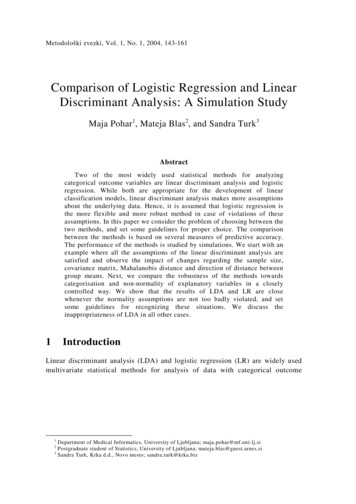
54Multivariate Logistic Regression ICU ExampleIDraw a causal diagram (DAG)typ?agesexserstaIArrow illustrates the direction of causalityICausality (and so arrows) must obey temporal orderingIAdmission type (emergency/elective) determined beforeservice type (medical/surgical)IFurther evidence that typ is the confounder: ser is notsignificant in the multivariate model
interpretation in univariate regression. I We dealt with 0 previously. I In general the coefficient k (corresponding to the variable X k) can be interpreted as follows: k is the additive change in the log-odds in favour of Y 1 when X k increases by 1 unit, while the other predictor variables remain unchanged.