Transcription
Spectral Analysis of Univariate and BivariateTime SeriesDonald B. PercivalSenior MathematicianApplied Physics LaboratoryHN–10University of WashingtonSeattle, WA 98195October 9, 1993
111.1IntroductionThe spectral analysis of time series is one of the most commonly used dataanalysis techniques in the physical sciences. The basis for this analysis is arepresentation for a time series in terms of a linear combination of sinusoidswith different frequencies and amplitudes. This type of representation iscalled a Fourier representation. If the time series is sampled at instances intime spaced t units apart and if the series is a realization of one portionof a real-valued stationary process {Xt } with zero mean, then we have therepresentation (due to Cramér [1]) f(N )Xt ei2πf t t dZ(f ),t 0, 1, 2, . . . ,(11.1) f(N )where f(N ) 1/(2 t) is the Nyquist frequency (if the units of t are measured in, say, seconds, then f(N ) is measured in Hertz (Hz), i.e., cycles persecond); i 1; and {Z(f )} is an orthogonal process (a complex-valuedstochastic process with quite special properties). This representation israther formidable at first glance, but the main idea is simple: since, by definition, ei2πf t t cos(2πf t t) i sin(2πf t t), Equation 11.1 says thatwe can express Xt as a linear combination of sinusoids at different frequencies f , with the sinusoids at frequency f receiving a random amplitudegenerated by the increment dZ(f ) Z(f df ) Z(f ) (here df is a smallpositive increment in frequency). The expected value of the squared magnitude of this random amplitude defines the spectral density function SX (·)for the stationary process {Xt } in the following way:E[ dZ(f ) 2 ] SX (f ) df, f(N ) f f(N )(the notation ‘E(X)’ refers to the expected value (mean) of the randomvariable (rv) X). Because dZ(f ) 2 is a nonnegative rv, its expectationmust be nonnegative, and hence the sdf SX (·) is a nonnegative function offrequency. Large values of the sdf tell us which frequencies in Equation 11.1contribute the most in constructing the process {Xt }. (We have glossed overmany details here, including the fact that a ‘proper’ sdf does not exist forsome stationary processes unless we allow use of the Dirac delta function.See Koopmans [2] or Priestley [3] for a precise statement and proof ofCramér’s spectral representation theorem or Section 4.1 of Percival andWalden [4] for a heuristic development.)Because {Xt } is a real-valued process, the sdf is an even function; i.e.,SX ( f ) SX (f ). Our definition for the sdf is ‘two-sided’ because it usesboth positive and negative frequencies, the latter being a nonphysical –but mathematically convenient – concept. Some branches of the physical
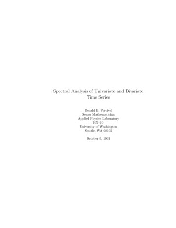
2sciences routinely use a ‘one-sided’ sdf that, in terms of our definition, isequal to 2SX (f ) over the interval [0, f(N ) ].Let us denote the τ th component of the autocovariance sequence (acvs)for {Xt } as Cτ,X ; i.e.,Cτ,X Cov(Xt , Xt τ ) E(Xt Xt τ )(the notation ‘Cov(X, Y )’ refers to the covariance between the rv’s X andY ). The spectral representation in Equation 11.1 can be used to derive theimportant relationship f(N )Cτ,X SX (f )ei2πf τ t df(11.2) f(N )(for details, see [4], Section 4.1). In words, SX (f ) is the (nonrandom) amplitude associated with the frequency f in the above Fourier representationfor the acvs {Cτ,X }. If we recall that C0,X is just the process variance, weobtain (by setting τ 0 in the above equation) f(N )V (Xt ) C0,X SX (f ) df f(N )(the notation ‘V (X)’ refers the variance of the rv X). The sdf thus represents a decomposition of the process variance into components attributableto different frequencies. In particular, if we were to run the process {Xt }through a narrow-band filter with bandwidth df centered at frequencies f ,the variance of the process coming out of the filter would be approximatelygiven by 2SX (f ) df (the factor of 2 arises because SX (·) is a two-sided sdf).Spectral analysis is an analysis of variance technique in which we portionout contributions to V (Xt ) across different frequencies. Because varianceis closely related to the concept of power, SX (·) is sometimes referred to asa power spectral density function.In this chapter we discuss estimation of the sdf SX (·) based upon a timeseries that can be regarded as a realization of a portion X1 , . . . , Xn of astationary process. The problem of estimating SX (·) in general is quitecomplicated, due both to the wide variety of sdf’s that arise in physicalapplications and also to the large number of specific uses for spectral analysis. To focus our discussion, we use as examples two time series that arefairly representative of many in the physical sciences; however, there aresome important issues that these series do not address and others that wemust gloss over due to space (for a more detailed exposition of spectralanalysis with a physical science orientation, see [4]). The two series areshown in Figure 11.1 and are a record of the height of ocean waves as a
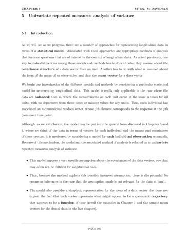
wave height (meters)wave height (meters)31(a)0-11(b)0-103570time (seconds)105140Figure 11.1: Plot of height of ocean waves versus time as measured bya wire wave gauge (a) and an infrared wave gauge (b). Both series werecollected at a rate of 30 samples per second. There are n 4096 datavalues in each series. (These series were supplied through the courtesy ofA. T. Jessup, Applied Physics Laboratory, University of Washington. Asof 1993, they could be obtained via electronic mail by sending a messagewith the single line ‘send saubts from datasets’ to the Internet addressstatlib@lib.stat.cmu.edu – this is the address for StatLib, a statisticalarchive maintained by Carnegie Mellon University).function of time as measured by two instruments of quite different design.Both instruments were mounted 6 meters apart on the same platform offCape Henry near Virginia Beach, Virginia. One instrument was a wire wavegauge, while the other was an infrared wave gauge. The sampling frequencyfor both instruments was 30 Hz (30 samples per second) so the samplingperiod is t 1/30 second and the Nyquist frequency is f(N ) 15 Hz.The series were collected mainly to study the sdf of ocean waves for frequencies from 0.4 to 4 Hz. The frequency responses of the instruments aresimilar only over certain frequency ranges. As we shall see, the infraredwave gauge inadvertently increases the power in the measured spectra byan order of magnitude at frequencies 0.8 to 4 Hz. The power spectra for
4the time series have a relatively large dynamic range (greater than 50 dB),as is often true in the physical sciences. Because the two instruments were6 meters apart and because of the prevalent direction of the ocean waves,there is a lead/lag relationship between the two series. (For more details,see Jessup et al. [5] and references therein.)11.2Univariate Time Series11.2.1The PeriodogramSuppose we have a time series of length n that is a realization of a portionX1 , X2 , . . . , Xn of a zero mean real-valued stationary process with sdf SX (·)and acvs {Cτ,X } (note that, if E(Xt ) is unknown and hence cannot beassumed to be zero, the common practice is to replace Xt with Xt X̄nprior to all other computations, where X̄ n1 t 1 Xt is the sample mean).Under a mild regularity condition (such as SX (·) having a finite derivativeat all frequencies), we can then writeSX (f ) t Cτ,X e i2πf τ t .(11.3)τ Our task is to estimate the sdf SX (·) based upon X1 , . . . , Xn . Equation 11.3 suggests the following ‘natural’ estimator. Suppose that, for τ n 1, we estimate Cτ,X via(p)Ĉτ,Xn τ 1 Xt Xt τ n t 1(the rationale for the superscript ‘(p)’ is explained below). The estimator(p)Ĉτ,X is known in the literature as the biased estimator of Cτ,X since itsexpected value is(p)E(Ĉτ,X ) n τ 1 τ E(Xt Xt τ ) 1 Cτ,X ,n t 1n(p)(11.4)(p)and hence E(Ĉτ,X ) Cτ,X in general. If we now decree that Ĉτ,X 0(p)for τ n and substitute the Ĉτ,X ’s for the Cτ,X ’s in Equation 11.3, weobtain the spectral estimator(p)ŜX (f ) tn 1 τ (n 1)Ĉτ,X e i2πf τ t .(p)(11.5)
5This estimator is known in the literature as the periodogram – hence thesuperscript ‘(p)’ – even though it is more natural to regard it as a function(p)of frequency f than of period 1/f . By substituting the definition for Ĉτ,Xinto the above equation and making a change of variables, we find also that 2 n t (p) i2πf t t ŜX (f ) Xt e(11.6) . n t 1Hence we can interpret the periodogram in two ways: it is the Fourier(p)transform of the biased estimator of the acvs (with Ĉτ,X defined to be zerofor τ n), and it is – to within a scaling factor – the squared modulus ofthe Fourier transform of X1 , . . . , Xn .Let us now consider the statistical properties of the periodogram. Ideally, we might like the following to be true:(p)1. E[ŜX (f )] SX (f ) (approximately unbiased);(p)2. V [ŜX (f )] 0 as n (consistent); and3. Cov[ŜX (f ), ŜX (f )] 0 for f f (approximately uncorrelated).(p)(p)The ‘tragedy of the periodogram’ is that in fact(p)1. ŜX (f ) can be a badly biased estimator of SX (f ) even for large samplesizes (Thomson [6] reports an example in which the periodogram isseverely biased for n 1.2 million data points) and(p)2. V [ŜX (f )] does not decrease to 0 as n (unless SX (f ) 0, acase of little practical interest).As a consolation, however, we do have that ŜX (f ) and ŜX (f ) are approximately uncorrelated under certain conditions (see below).We can gain considerable insight into the nature of the bias in theperiodogram by studying the following expression for its expected value: f(N ) t sin2 (nπf t)(p)E[ŜX (f )] F(f f )SX (f ) df , with F(f ) n sin2 (πf t) f(N )(11.7)(for details, see [4], Section 6.3). The function F(·) is known as Fejér’s kernel. We also call it the spectral window for the periodogram. Figure 11.2(a)shows F(f ) versus f with f(N ) f f(N ) for the case n 32 with t 1so that f(N ) 1/2 (note that F( f ) F(f ); i.e., Fejér’s kernel is an evenfunction). Figure 11.2(b) plots 10 · log10 (F(f )) versus f for 0 f 1/2(p)(p)
62(a)20(b)06-200-40-0.50.0f0.50.00.5fFigure 11.2: Fejér’s kernel for sample size n 16 with f(N ) 1/2.(i.e., F(·) on a decibel scale). The numerator of Equation 11.7 tells us thatF(f ) 0 when the product nf t is equal to a nonzero integer – thereare 16 of these nulls evident in 11.2(b). The nulls closest to zero frequencyoccur at f 1/(n t) 1/32. Figure 11.2(a) indicates that F(·) isconcentrated mainly in the interval of frequencies between these two nulls,the region of the ‘central lobe’ of Fejér’s kernel. A convenient measure of 1/(N t) f(N )this concentration is the ratio 1/(N t) F(f ) dfF(f ) df . An easy f(N )exercise shows that the denominator is unity for all n, while – to two decimal places – the numerator is equal to 0.90 for all n 13. As n ,the length of the interval over which 90% of F(·) is concentrated shrinks tozero, so in the limit Fejér’s kernel acts like a Dirac delta function. If SX (·)(p)is continuous at f , Equation 11.7 tells us that limn E[ŜX (f )] SX (f );i.e., the periodogram is asymptotically unbiased.While this asymptotic result is of some interest, for practical applications we are much more concerned about possible biases in the periodogramfor finite sample sizes n. Equation 11.7 tells us that the expected value ofthe periodogram is given by the convolution of the true sdf with Fejér’skernel. Convolution is often regarded as a smoothing operation. From(p)this viewpoint, E[ŜX (·)] should be a smoothed version of SX (·) – hence,(p)if SX (·) is itself sufficiently smooth, E[ŜX (·)] should closely approximateSX (·). An extreme example of a process with a smooth sdf is white noise.(p)Its sdf is constant over all frequencies, and in fact E[ŜX (f )] SX (f ) fora white noise process.For sdf’s with more structure than white noise, we can identify twosources of bias in the periodogram. The first source is often called a lossof resolution and is due to the fact that the central lobe of Fejér’s kernel
7will tend to smooth out spectral features with widths less than 1/(n t).Unfortunately, unless a priori information is available (or we are willingto make a modeling assumption), the cure for this bias is to increase thesample size n, i.e., to collect a longer time series, the prospect of whichmight be costly or – in the case of certain geophysical time series spanningthousands of years – impossible within our lifetimes.The second source of bias is called leakage and is attributable to thesidelobes in Fejér’s kernel. These sidelobes are prominently displayed inFigure 11.2(b). Figure 11.3 illustrates how these sidelobes can induce bias inthe periodogram. The thick curve in Figure 11.3(a) shows an sdf plotted ona decibel scale from f f(N ) to f f(N ) with f(N ) 1/2 (recall that thesdf is symmetric about 0 so that SX ( f ) SX (f )). The thin bumpy curveis Fejér’s kernel for n 32, shifted so that its central lobe is at f 0.2. Theproduct of this shifted kernel and the sdf is shown in Figure 11.3(b) (again(p)on a decibel scale). Equation 11.7 says that E[ŜX (0.2)] is the integralof this product. The plot shows this integral to be mainly determined by(p)values close to f 0.2; i.e., E[ŜX (0.2)] is largely due to the sdf at valuesclose to this frequency, a result that is quite reasonable. Figures 11.3(c)(p)and (d) show the corresponding plots for f 0.4. Note that E[ŜX (0.4)] issubstantially influenced by values of SX (·) away from f 0.4. The problemis that the sidelobes of Fejér’s kernel are interacting with portions of the sdfthat are the dominant contributors to the variance of the process so that(p)(p)E[ŜX (0.4)] is biased upwards. Figure 11.3(e) shows a plot of E[ŜX (f )]versus f (the thin curve), along with the true sdf SX (·) (the thick curve).While the periodogram is essentially unbiased for frequencies satisfying0.1 f 0.35, there is substantial bias due to leakage at frequenciesclose to f 0 and f 1/2 (in the latter case, the bias is almost 40 dB,i.e., 4 orders of magnitude).While it is important to know that the periodogram can be severelybiased for certain processes, it is also true that, if the true sdf is sufficiently(p)lacking in structure (i.e., ‘close to white noise’), then SX (·) and E[ŜX (·)]can be close enough to each other so that the periodogram is essentiallybias free. Furthermore, even if leakage is present, it might not be of importance in certain practical applications. If, for example, we were performinga spectral analysis to determine the height and structure of the sdf in Figure 11.3 near f 0.2, then the bias due to leakage at other frequencies isof little concern.If the portions of the sdf affected by leakage are in fact of interest or ifwe are carrying out a spectral analysis on a time series for which little isknown a prior about its sdf, we need to find ways to recognize when leakageis a problem and, if it is present, to minimize it. As is the case for loss of
.5 -0.50.0f(e)0.5(f)dB200-20-400.00.5 0.0f0.5fFigure 11.3: Illustration of leakage (plots (a) to (e)). The Nyquist frequencyf(N ) here is taken to be 1/2. Plot (f) shows the alleviation of leakage viatapering and is discussed in Section 11.2.2.
9resolution, we can decrease leakage by increasing the sample size (moredata can solve many problems!), but unfortunately a rather substantialincrease might be required to obtain a periodogram that is essentially freeof leakage. Consider again the sdf used as an example in Figure 11.3. Evenwith a 32 fold increase in the sample size from n 32 to 1024, there is still(p)more than a 20 dB difference between E[ŜX (0.5)] and SX (0.5).If we regard the sample size as fixed, there are two well-known waysof decreasing leakage, namely, data tapering and prewhitening. Both ofthese techniques have a simple interpretation in terms of the integral inEquation 11.7. On the one hand, tapering essentially replaces Fejér’s kernelF(·) by a function with substantially reduced sidelobes; on the other hand,prewhitening effectively replaces the sdf SX (·) with one that is closer towhite noise. Both techniques are discussed in the next subsection.11.2.2Correcting for BiasTaperingFor a given time series X1 , X2 , . . . , Xn , a data taper is a finite sequenceh1 , h2 , . . . , hn of real-valued numbers. The product of this sequence andthe time series, namely, h1 X1 , h2 X2 , . . . , hn Xn , is used to create a directspectral estimator of SX (f ), defined as 2 n (d)ŜX (f ) t ht Xt e i2πf t t .(11.8) t 1 Note that, if we let ht 1/ n for all t (the so-called rectangular data(d)taper), a comparison of Equations 11.8 and 11.6 tells us that ŜX (·) reduces(d)to the periodogram. The acvs estimator corresponding to ŜX (·) is justn τ (d)Ĉτ,X n τ (d)ht Xt ht τ Xt τ , and so E(Ĉτ,X ) Cτ,Xt 1 ht ht τ .t 1(11.9)If we insist thatbe an unbiased estimator of the process variance C0,X , nthen we obtain the normalization t 1 h2t 1 (note that the rectangulardata taper satisfies this constraint).The rationale for tapering is to obtain a spectral estimator whose expected value is close to SX (·). In analogy to Equation 11.7, we can expressthis expectation as f(N )(d)E[ŜX (f )] H(f f )SX (f ) df ,(11.10)(d)Ĉ0,X f(N )
10.4(a)20(b)0-20.-40-60.0.4(c).0 . .4.0.4. . . . .(d)0.-20.-40.-60. . -80(e)20. . . . . .-20.-40.-60. .(h)-20.-40.-60.33t-80200.(f)0.(g).0 . . .0-8020-800.00.5fFigure 11.4: Four data tapers (left-hand column of plots) and their spectralwindows (right-hand column) for a sample size of n 32. From top tobottom, the tapers are the rectangular taper, the Hanning taper, the dpssdata taper with nW 2/ t and the dpss data taper with nW 3/ t(here t 1).
11where H(·) is proportional to the squared modulus of the Fourier transformof the ht ’s and is called the spectral window for the direct spectral estimator(d)ŜX (·) (just as we called Fejér’s kernel the spectral window for the periodogram). The claim is that, with a proper choice of ht ’s, we can producea spectral window that offers better protection against leakage than Fejér’skernel. Figure 11.4 supports this claim. The left-hand column of plotsshows four data tapers for sample size n 32, while the right-hand plotsshow the corresponding spectral windows. For the sake of comparison, thedata taper in 11.4(a) is just the rectangular data taper, so the corresponding spectral window is Fejér’s kernel (cf. Figure 11.2(b)). The data taperin 11.4(c) is the well-known Hanning data taper , which we define to beht 2/3(n 1) [1 cos (2πt/(n 1))] for t 1, . . . , n (there are other– slightly different – definitions in the literature). Note carefully the shapeof the corresponding spectral window in 11.4(d): its sidelobes are considerably suppressed in comparison to those of Fejér’s kernel, but the widthof its central lobe is markedly larger. The convolutional representation(d)for E[ŜX (f )] given in Equation 11.10 tells us that an increase in centrallobe width can result in a loss of resolution when the true sdf has spectralfeatures with widths smaller than the central lobe width. This illustratesone of the tradeoffs in using a data taper, namely, that tapering typicallydecreases leakage at the expense of a potential loss of resolution.A convenient family of data tapers that facilitates the tradeoff betweensidelobe suppression and the width of the central lobe is the discrete prolate spheroidal sequence (dpss) tapers. These tapers arise as the solution tothe following ‘concentration’ problem. Suppose we pick a number W that– roughly speaking – we think of as half the desired width of the centrallobe of the resulting spectral window (typically 1/(n t) W 4/(n t)although larger values for W are sometimes useful). n Under the requirementthat the taper must satisfy the normalization t 1 h2t 1, the dpss taperis, by definition, the taper whose corresponding spectral window is as concentrated as possible in the frequency interval [ W, W ] in the sense that W fthe ratio W H(f ) df f(N(N) ) H(f ) df is as large as possible (note that, ifH(·) were a Dirac delta function, this ratio would be unity). The quantity2W is sometimes called the resolution bandwidth. For a fixed W , the dpsstapers have sidelobes that are suppressed as much as possible as measuredby the concentration ratio. To a good approximation (Walden [7]), thedpss tapers can be calculated as ht C I0 (W 1 (1 gt )2 )/I0 (W ) fort 1, . . . , n, where C is a scaling constant used to force the normalizationh2t 1; W πW (n 1) t; gt (2t 1)/n; and I0 (·) is the modifiedBessel function of the first kind and zeroth order (this can be computedusing the Fortran function bessj0 in Section 6.5 of Press et al. [8]).
12Figures 11.4(e) and (g) show dpss tapers for n 32 and with W setsuch that nW 2/ t and nW 3/ t, while plots (f) and (h) show thecorresponding spectral windows H(·) (the quantity 2nW is known as theduration-bandwidth product). The vertical lines in the latter two plotsmark the locations of W . Note that in both cases the central lobe ofH(·) is approximately contained between [ W, W ]. As expected, increasingW suppresses the sidelobes and hence offers increasing protection againstleakage. A comparison of the spectral windows for the Hanning and nW 2/ t dpss tapers (Figures 11.4(d) and (f)) shows that, whereas their centrallobes are comparable, their sidelobe structures are quite different. Whilespecific examples can be constructed in which one of the tapers offers betterprotection against leakage than the other, generally the two tapers are quitecomparable in practical applications. The advantage of the dpss tapers isthat, if, say, use of an nW 2/ t dpss taper produces a direct spectralestimator that still suffers from leakage, we can easily obtain a greaterdegree of protection against leakage by merely increasing nW beyond 2/ t.The choice nW 1/ t yields a spectral window with a central lobe closelyresembling that of Fejér’s kernel but with sidelobes about 10 dB smaller.Let us now return to the example of Figure 11.3. Recall that the thin(p)curve in 11.3(e) shows E[ŜX (f )] versus f for a process with an sdf given(d)by the thick curve. In 11.3(f) the thin curve now shows E[ŜX (·)] for adirect spectral estimator employing an nW 2/ t dpss taper. Note thattapering has produced a spectral estimator that is overall much closer inexpectation to SX (·) than the periodogram is; however, mainly due to the(d)small sample n 32, ŜX (·) still suffers from leakage at some frequencies(about 10 dB at f 0.5).In practical situations, we can determine if leakage is present in theperiodogram by carefully comparing it with a direct spectral estimate constructed using a dpss data taper with a fairly large value of W . As anexample, Figure 11.5(a) shows the periodogram for the wire wave gaugetime series shown in Figure 11.1. Since these data were collected mainly toinvestigate the rolloff rate of the sdf from 0.8 to 4 Hz, we have only plottedthe low frequency portion of the periodogram. Figure 11.5(b) shows a directspectral estimate for which we have used a dpss taper with nW 4/ t.Note that the direct spectral estimate is markedly lower than the periodogram at frequencies with a relatively small contribution to the overallvariance – for example, the former is about 10 dB below the latter at frequencies close to 4 Hz. This pattern is consistent with what we wouldexpect to see when there is leakage in the periodogram. Increasing nWbeyond 4/ t to, say, 6/ t and comparing the resulting direct direct spectral estimate with that of Figure 11.5(b) indicates that the nW 4/ t
13estimated sdf (meters2/Hz in frequency (Hz)4 0123frequency (Hz)4Figure 11.5: Periodogram (plot (a)) and a direct spectral estimate (plot (b))using an nW 4/ t dpss data taper for the wire gauge time series ofFigure 1(a). Both estimates are plotted on a decibel scale. The smallsubplots in the upper right-hand corner of each plot give an expanded viewof the estimators at 0 f 0.5 Hz (the vertical scales of the subplots arethe same as those of the main plots).estimate is essentially leakage free; on the other hand, an examination ofan nW 1/ t direct spectral estimate indicates that it is also essentiallyleakage free for the wave gauge series. In general, we can determine an appropriate degree of tapering by carefully comparing the periodogram anddirect spectral estimates corresponding to dpss tapers with different valuesof nW . If the periodogram proves to suffer from leakage (as it often does inthe physical sciences), we then seek a leakage free direct spectral estimateformed using as small a value of W – and hence nW – as possible. A smallW is desirable from 2 viewpoints: first, resolution typically decreases as Wincreases, and, second, the distance in frequency between approximatelyuncorrelated spectral estimates increases as W increases (this causes a lossin degrees of freedom when we subsequently smooth across frequencies –see Section 11.2.3 for details).In checking for the presence of leakage, comparison between different
14spectral estimates is best done graphically in the following ways:1. by comparing spectral estimates side by side (as in Figure 11.5) or ontop of each other using different colors;2. by plotting the ratio of two spectral estimates on a decibel scale versusfrequency and searching for frequency bands over which an averageof this ratio is nonzero (presumably a statistical test could be devisedhere to assess the significance of departures from zero); and(p)(d)3. by constructing scatter plots of, say, ŜX (f ) versus ŜX (f ) for f ’sin a selected band of frequencies and looking for clusters of pointsconsistently above a line with unit slope and zero intercept.The use of interactive graphical displays would clearly be helpful in determining the proper degree of tapering (Percival and Kerr [9]).PrewhiteningThe loss of resolution and of degrees of freedom inherent in tapering canbe alleviated considerably if we can prewhiten our time series. To explainprewhitening, we need the following result from the theory of linear timeinvariant filters. Given any set of p 1 real-valued numbers a0 , a1 , . . . , ap ,we can filter X1 , . . . , Xn to obtainWt p ak Xt k ,t p 1, . . . , n.(11.11)k 0The filtered process {Wt } is a zero mean real-valued stationary process withan sdf SW (·) related to SX (·) via2SW (f ) A(f ) SX (f ), where A(f ) p ak e i2πf k t .(11.12)k 0A(·) is the transfer function for the filter {ak }. The idea behind prewhitening is to find a set of ak ’s such that the sdf SW (·) has substantially lessstructure than SX (·) and ideally is as close to a white noise sdf as possible.If such a filter can be found, we can easily produce a leakage-free direct spec(d)tral estimate ŜW (·) of SW (·) requiring little or no tapering. Equation 11.12(pc)(d)2tells us that we can then estimate SX (·) using ŜX (f ) ŜW (f ) A(f ) ,where the superscript ‘(pc)’ stands for postcolored.The reader might note an apparent logical contradiction here: in orderto pick a reasonable set of ak ’s, we must know the shape of SX (·), the very
15function we are trying to estimate! There are two ways around this inherentdifficulty. In many cases, there is enough prior knowledge concerning SX (·)from, say, previous experiments so that, even though we don’t know theexact shape of the sdf, we can still design an effective prewhitening filter. Inother cases we can create a prewhitening filter based upon the data itself.A convenient way of doing this is by fitting autoregressive models of orderp (hereafter AR(p)). In the present context, we postulate that, for somereasonably small p, we can model Xt as a linear combination of the p priorvalues Xt 1 , . . . , Xt p plus an error term; i.e,Xt p φk Xt k Wt ,t p 1, . . . , n,(11.13)k 1where {Wt } is an ‘error’ process with an sdf SW (·) that has less structure than SX (·). The stipulation that p be small is desirable because theprewhitened series {Wt } will be shortened to length n p. The above equation is a special case of Equation 11.11, as can be seen by letting a0 1and ak φk for k 0.For a given p, we can obtain estimates of the φk ’s from our time seriesusing a number of different methods (see [4], Chapter 9). One method thatgenerally works well is Burg’s algorithm, a computationally efficient wayof producing estimates of the φk ’s that are guaranteed to correspond toa stationary process. The Fortran subroutine memcof in [8], Section 13.6,implements Burg’s algorithm (the reader should note that the time seriesused as input to memcof is assumed to be already adjusted for any nonzeromean value).Burg’s algorithm (or any method that estimates the φk ’s in Equation 11.13) is sometimes used by itself to produce what is known as anautoregressive spectral estimate (this is one form of parametric spectralestimation). If we let φ̄k represent Burg’s estimate of φk , then the corresponding autoregressive spectral estimate is given by(ar)S̄X (f ) 1 pσ̄p2 tk 1 2 ,φ̄k e i2πf k t (11.14)where σ̄p2 is an estimate of the variance of {Wt }. The key difference between an autoregressive spectral estimate and prewhitening is in the useof Equation 11.13: the former assumes the process {Wt } is exactly whitenoise, whereas the latter merely postulates {Wt } to have an sdf with lessstructure than {Xt }. Autoregressive spectral estimation works well formany time series, but it depends heavily on a proper choice of the order p;(ar)moreover, simple ap
Spectral Analysis of Univariate and Bivariate Time Series DonaldB.Percival SeniorMathematician AppliedPhysicsLaboratory HN-10 UniversityofWashington Seattle,WA98195 October9,1993. 1 . analysis with a physical science orientation, see [4]). The two series are shown in Figure 11.1 and are a record of the height of ocean waves as a. 3-1 0