Transcription
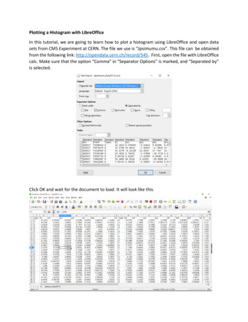
Plotting a Histogram with LibreOfficeIn this tutorial, we are going to learn how to plot a histogram using LibreOffice and open datasets from CMS Experiment at CERN. The file we use is “Jpsimumu.csv”. This file can be obtainedfrom the following link: http://opendata.cern.ch/record/545. First, open the file with LibreOfficecalc. Make sure that the option “Comma” in “Separator Options” is marked, and “Separated by”is selected.Click OK and wait for the document to load. It will look like this.
We’re only going to use the values for the mass. Select the rest on the columns by clicking onthem, then right-click and delete them using the “Delete Columns” option of the menu thatappears.You can add a new sheet by clicking thebutton in the lower left-hand side of the screen.Rename this sheet Mass Histogram by double clicking on the name. There are approximatelyalmost 32 thousand values for the invariant mass.Now we are going to calculate the minimum and the maximum mass values in this file. You cando this by using the function MIN( ), and selecting all the mass values in the file. It is easier andquicker to just write the names of the first and last cell in the parenthesis.
Click Enter, and the minimum value for the mass will be shown on the screen. Now we have todo the same to calculate the maximum value, but use the function MAX( ) instead. We also needto know the exact number of values we have in this file. For this we can use the function COUNT().Our histogram will begin from 2.0 GeV and end in 5.0 GeV in order to include all the values thatwe have in our data.We can now begin to create our classes for the histogram. In the column next to the mass column,write the heading “Bins” and then numbers going from 2.0 to 5.0 in steps of 0.10 . This will allowto better visualize the data and see what particles appear in our histogram.You can easily create these values by writing the first three numbers, selecting them and thensliding until we see the last value we want (5.0, shown in the picture below).
Next to the “Bins” heading now write a “Frequency” heading. Now we are going to use theFrequency function. Click on the cell below the “Frequency” heading, then in the toolbar, select“Insert”, then “Function”.
A window will pop-up. There, select the function category “Array”, and the function“FREQUENCY”, as shown in the picture below. Click on Next.A window like this one will appear:
Click on thebutton next “data”. From there you can select all the mass values manually withthe mouse, but it is easier to write the range. Include the range in the window and click Enter.You will return to the previous window. There you can do the same and include all the “Bins”values in “classes”.Once your screen looks like this, you can click OK. The values of the frequencies will appear.
You can see that the first value of the frequency is 0. This is because the bin value to the left isthe upper limit of the class, that is, the function will only count values of the mass that are lessthan 2.0. As we have no values of the mass that are less than 2.0, we get a frequency of 0 for thisclass.We can now make our histogram. Select in the toolbar the option “Insert”, then “Chart”. Awindow like this one will appear:
There, you can decide if you want to plot your values as columns or dots. We can select thecolumn option and click next.In this window, you can select the values that will be used for the histogram. Make sure that theoptions “First column as label” and “First row as label” are marked, and select the option “Dataseries in columns”. You can select the values for the histogram manually as explained before withthebutton or you can write down the range. You can now click finish to see your histogram.It will look something like this:Notice there’s a big peak at approximately 3.1 GeV, and there seems to be a smaller peak at 3.7GeV. Knowing that our file contains only events where to muons have been detected, we canthen find out which particle has a mass of approximately 3.1 GeV and decays into two muons.
Such particle is the J/ψ Meson. One other particle that has a mass of approximately 3.7 GeV anddecays into two muons is the ψ(2S) meson.ExercisePlot invariant mass histograms using different data sets. You can find more data sets at thefollowing link: http://opendata.cern.ch/record/545.
In this window, you can select the values that will be used for the histogram. Make sure that the options "First column as label" and "First row as label" are marked, and select the option "Data series in columns". You can select the values for the histogram manually as explained before with the button or you can write down the range.