Transcription
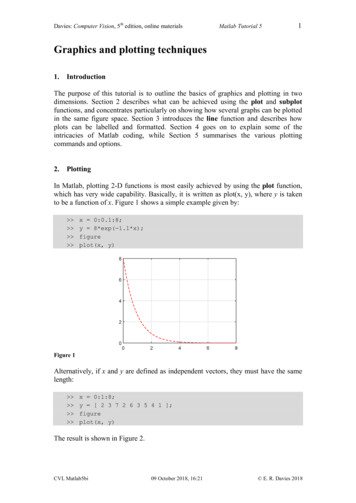
Davies: Computer Vision, 5th edition, online materialsMatlab Tutorial 51Graphics and plotting techniques1.IntroductionThe purpose of this tutorial is to outline the basics of graphics and plotting in twodimensions. Section 2 describes what can be achieved using the plot and subplotfunctions, and concentrates particularly on showing how several graphs can be plottedin the same figure space. Section 3 introduces the line function and describes howplots can be labelled and formatted. Section 4 goes on to explain some of theintricacies of Matlab coding, while Section 5 summarises the various plottingcommands and options.2.PlottingIn Matlab, plotting 2-D functions is most easily achieved by using the plot function,which has very wide capability. Basically, it is written as plot(x, y), where y is takento be a function of x. Figure 1 shows a simple example given by: x 0:0.1:8;y 8*exp(-1.1*x);figureplot(x, y)Figure 1Alternatively, if x and y are defined as independent vectors, they must have the samelength: x 0:1:8;y [ 2 3 7 2 6 3 5 4 1 ];figureplot(x, y)The result is shown in Figure 2.CVL Matlab5bi09 October 2018, 16:21 E. R. Davies 2018
Davies: Computer Vision, 5th edition, online materialsMatlab Tutorial 52Figure 2Complete script for Figure 2. For a detailed explanation of the various functions used in this and otherscripts, see Section 3.x linspace(0,8,9);y [2 3 7 2 6 3 5 4 4 3 1])axis([0 8 0 8])set(gca, 'fontsize',14)set(gca, 'XTick',[0 2 4 6 8])set(gca, 'YTick',[0 2 4 6 8])set(gca, 'LineWidth',1.0)grid onIn the following example, the total number of data points is 7, and the resultinggraph is a 6-line approximation to the cosine curve. theta 0:15:90;y cos(theta*pi/180);figureplot(theta, y)Figure 3In fact, it is usually more transparent to use the linspace operator as the basis forplotting operations: this has arguments representing the start x1 and end xn values andCVL Matlab5bi09 October 2018, 16:21 E. R. Davies 2018
Davies: Computer Vision, 5th edition, online materialsMatlab Tutorial 53the total number of points n created within the range x1 to xn; note that n includes thestart and end points, and is therefore not equal to the number of intervals between thestart and end points. In fact, identically the same graph (Figure 3) can be generatedusing the linspace operator: theta linspace(0,90,7);y cos(theta*pi/180);figureplot(theta, y)If the argument n is omitted, the function defaults to 100. Interestingly, this isoften a good compromise value for plotting functions.Note that to create a new figure, the command figure must appear before the plotfunction is applied, as indicated in the above examples.A useful facility is that of being able to include several graphs in the same plotarea, merely by including several sets of arguments in the plot brackets: x linspace(0,8);y1 8*exp(-1.1*x);y2 x;y3 1.5*y1 .* y2;figureplot(x, y1, x, y2, x, y3)Figure 4Note how the complete script for Figure 4 includes not only the plotted functionsbut also information on the plotting colours, plotting characteristics, axes, tick marksand instructions to include a grid in the graphics box.CVL Matlab5bi09 October 2018, 16:21 E. R. Davies 2018
Davies: Computer Vision, 5th edition, online materialsMatlab Tutorial 54Complete script for Figure 4x linspace(0,8);y1 8*exp(-1.1*x);y2 x;y3 1.5*y1 .* eWidth',1.2)pbaspect([4 3 1])axis([0 8 0 8])set(gca, 'fontsize',14)set(gca, 'XTick',[0 2 4 6 8])set(gca, 'YTick',[0 2 4 6 8])set(gca, 'LineWidth',1.0)grid onAn alternative is to make use of the hold on function: this has been incorporated intothe following code, generating exactly the same figure: x linspace(0,8);y1 8*exp(-1.1*x);y2 x;y3 1.5*y1 .* y2;figureplot(x, y1)hold onplot(x, y2)plot(x, y3)After a hold on operation, a new plot is added without deleting any old ones, soprevious plots in the current graphics window are retained. After a hold off operation,a new plot replaces any old ones, so previous plots in the current graphics window areeliminated. Note that once asserted, a hold state continues until a hold off operation isapplied.Whereas it is useful to be able to show multiple graphs 'on top of each other' inthe same plot space, it is often preferable to display them separately in an array ofsubplots, as in Figure 5. This is achieved with the following set of commands, inwhich we define several sets of axes and arrange them in a regular array:CVL Matlab5bi09 October 2018, 16:21 E. R. Davies 2018
Davies: Computer Vision, 5th edition, online materials Matlab Tutorial 55x linspace(0,8);y1 8*exp(-1.1*x);y2 x;y3 1.5*y1 .* y2;figureaxes1 subplot(2,2,1);plot(axes1, x, y1)axes2 subplot(2,2,2);plot(axes2, x, y2)axes3 subplot(2,2,3);plot(axes3, x, y3)axes4 subplot(2,2,4);plot(axes4, x, y1, x, y2, x, y3)Figure 5Complete script for Figure 5x linspace(0,8);y1 8*exp(-1.1*x);y2 x;y3 1.5*y1 .* y2;figureset(gca, 'fontsize',28)set(gca, 'LineWidth',1.5)axes1 .0)axis([0 8 0 8]); pbaspect([4 3 1]); grid onaxes2 .0)axis([0 8 0 8]); pbaspect([4 3 1]); grid onaxes3 0)axis([0 8 0 8]); pbaspect([4 3 1]); grid onaxes4 y3,'k-','LineWidth',1.0)axis([0 8 0 8]); pbaspect([4 3 1]); grid onCVL Matlab5bi09 October 2018, 16:21 E. R. Davies 2018
Davies: Computer Vision, 5th edition, online materialsMatlab Tutorial 56When using the subplot function, the three arguments appearing in the bracketsare respectively the number of rows of subplots, the number of column subplots andthe number in the sequence (in which we number along the first row and then alongthe other rows in turn).So far, we have only considered graphs in which y is plotted as a function of x—which is a strategy that only works for single-valued functions. However, it is easy togeneralise it to other types of function. This is achieved by using parametric forms forsuch functions. For example, Figure 6 shows that a circle is easily generated by takingangle theta relative to its centre and employing sine and cosine functions: theta linspace(0,360);x cos(theta);y sin(theta);figureplot(x, y)Figure 6Complete script for Figure 6theta linspace(0,360);x cos(theta*pi/180);y ,1.2)axis squareaxis([-1 1 -1 1])set(gca, 'fontsize',14)set(gca, 'LineWidth',1.0)grid on3.Labelling and formatting graphsClearly, it can be confusing for several functions to be plotted in the same 2-D space,so it is useful for them to be distinguished by various line styles and colors, and alsoto have the capability for adding discrete markers to represent specific points. All thiscan be achieved by including line and marker specifications alongside the plotarguments. In fact, we can generalise the previous plot instruction to the following:CVL Matlab5bi09 October 2018, 16:21 E. R. Davies 2018
Davies: Computer Vision, 5th edition, online materials7Matlab Tutorial 5 plot(x, y1, linespec1, x, y2, linespec2, x, y3, linespec3)This may be implemented using the following simple notation that will be describedbelow: figure plot(x, y1, 'r--', x, y2, 'g:', x, y3, 'b-')Importantly, the line specification is conveniently expressed in a few characterssuch as '--ro', where '--' means that the line is dashed, 'r' means that the color is red,and 'o' means that the marker is to be a circle. Note that: the whole of the specification is expressed in single quotes which include anoptional line specification L, an optional marker specification M, and an optionalcolor specification CL, M and C can be written in any orderif only L is included, only a line is drawnif only M is included, only markers are drawnif both L and M are included, both a line and markers are drawn, with the samecolorif neither L nor M is included, a default line is drawn without any markers.The highly compact representation described above is made possible by use of acleverly chosen set of codes, including the following:line styledasheddotteddash dotsolid squarediamondpentagram (5-point star)hexagram (6-point star)pluscrossasteriskN-pointing triangleS-pointing triangleE-pointing triangleW-pointing trianglecode.osdph x* v (Note that, to avoid confusion with blue, black is represented by its last letter.)To provide further guidance, most of the codes listed above were used to generateFigure 7 and are included in its Matlab script.There are a few additional refinements to the above description. For example, toavoid all the data points appearing as markers, marker indices can be specified byincluding the following additional information in the line specification:CVL Matlab5bi09 October 2018, 16:21 E. R. Davies 2018
Davies: Computer Vision, 5th edition, online materialsMatlab Tutorial 58'MarkerIndices', 1:n:length(y): this ensures that only every nth data point will be amarker.Markers such as squares and circles can have different boundary (edge) and fill(face) colors. These can be assigned using the following name–value pair extensionsto the line specification: 'MarkerEdgeColor', 'g' and 'MarkerFaceColor', 'b'.The widths of lines can be specified by using the 'LineWidth' parameter, which isset using point values, with a default value of 0.5: note that this parameter alsomodifies the boundary widths of markers. Finally, marker size can also be set usingthe name–value pair, 'MarkerSize', m, where m is proportional to the area of themarker: it has a default value of 6.Figure 7Complete script for Figure 7x linspace(0,8,9);y [2 3 7 2 6 3 5 4 1];figuregrid on; box onhold t(x,y*0.4,':r ','MarkerSize',5,'LineWidth',1.2)plot(x,y*0.3,'g 'w')pbaspect([4 3 1])axis([0 8 0 8])set(gca, 'fontsize',14)set(gca, 'XTick',[0 2 4 6 8])set(gca, 'YTick',[0 2 4 6 8])set(gca, 'LineWidth',1.0)Interestingly, color can be specified more accurately using RGB triplet values:these must each be in the range [0, 1]. The table below gives the equivalent RGBtriplet values for the above eight common colors:CVL Matlab5bi09 October 2018, 16:21 E. R. Davies 2018
Davies: Computer Vision, 5th edition, online ackcodergbcmywkMatlab Tutorial 59RGB triplet[1 0 0][0 1 0][0 0 1][0 1 1][1 0 1][1 1 0][1 1 1][0 0 0]Plots may be augmented by including titles, labels along the x and y axes, andsimilarly for subplots:title('2-D line plot')xlabel('x-axis')ylabel('y-axis')title(axes1, '2-D line subplot1')xlabel(axes1, 'subplot1 x-axis')ylabel(axes1, 'subplot1 y-axis')Many possibilities exist for formatting titles and labels. In particular, thefollowing are important. Font size, font weight and font color can be modified usingthe usual name–value pair arguments, e.g., xlabel('x-axis', 'FontSize', 12,'FontWeight', 'bold', 'Color', 'g'). Here, FontSize specifies the font size in points, with11 points being the default for labels and 10 points being the default for axes. Inaddition, 'FontName' specifies the name of the font (e.g., 'Courier'), which defaults toHelvetica.Labelling can include Greek letters and other characters generated by using TeXmarkup—e.g., \pi, \leq, \theta, and so on. Note that superscripts and subscripts can beincluded using the TeX ' ' and ' ' notation, accompanied by curly brackets if morethan one character is to be inserted ( { } and { }). TeX markup also generalises theinclusion of font weights (\bf (bold), \rm (normal), \it (italic)), font sizes(\fontsize{8} .), font colors using both standard colors (\color{magenta}, .), andRGB triplets (\color[rgb]{0.1, 0.2, 0.3}, .).Note that variable names can be converted to strings using the num2str function.This is frequently useful, e.g., for labelling subplots automatically, as in Figure 8: x linspace(0,8);figurefor i 1:4axesi subplot(2,2,i);y exp(-i/2*x);plot(axesi, x, y)title( axesi, [ 'scale factor ' num2str(i/2) ])% the square brackets act to concatenate the two stringsendCVL Matlab5bi09 October 2018, 16:21 E. R. Davies 2018
Davies: Computer Vision, 5th edition, online materialsMatlab Tutorial 510Figure 8Figure 9Figure 10Notice that unnecessary space between the four subplots can be eliminated by usingthe get function to access the subplot position vector (this has four elements [left,bottom, width, height]), adjusting the left and bottom values, and finally applying thenew position using the set function: the result is shown in Figure 9; the completeMatlab script appears below. Additionally, if (as sometimes happens in practice) theaxes and title options are not needed, further space can be removed as shown inFigure 10: note that the axis off option eliminates the axes, tick marks and labels. InFigure 10 the position adjustments were set at 0.04, 0.03—exactly double those forFigure 9.CVL Matlab5bi09 October 2018, 16:21 E. R. Davies 2018
Davies: Computer Vision, 5th edition, online materialsMatlab Tutorial 511Complete script for Figure 9x linspace(0,8);figureset(gca, 'fontsize',28)for i 1:4axesi subplot(2,2,i);y exp(-i/2*x);p get(axesi, 'position');if i 1 i 3, p(1) p(1) 0.02; endif i 2 i 4, p(1) p(1) - 0.02; endif i 1 i 2, p(2) p(2) - 0.015; endif i 3 i 4, p(2) p(2) 0.015; endset(axesi, 'position', p)plot(axesi,x,y,'-k','LineWidth',1.0)set(gca, 'XTick',([0 2 4 6 8]))set(gca, 'YTick',([0 0.2 0.4 0.6 0.8 1]))title(axesi,['scale factor ' num2str(i/2) ])endOne other function that is often useful is the line function, which is aimed atjoining single pairs of points. As such it could be regarded as replacing the plotfunction, which is aimed at joining sequences of points. However, it can be useful forsimplicity: for example, it can be used to draw a line right across a set of existingplots without deleting other objects or changing the axis settings. A simple exampleis: x [1 8];y [3 7];line(x, y, '--dg')% here the line end points are (1,3) and (8,7)More elaborate examples are shown in Figures 11 and 12, together with theirassociated Matlab scripts. Interestingly, more relevant lines and curves often need tobe plotted later so that they can be seen to partially overwrite earlier plots—which canbe important to the appearance of the final figure, as happens in Figures 11 and 12.CVL Matlab5bi09 October 2018, 16:21 E. R. Davies 2018
Davies: Computer Vision, 5th edition, online materialsMatlab Tutorial 512Figure 11. This figure shows how plots, lines, axes, scales and labelling can be put together to form avital illustration. It is essentially the same as Figure 14.14 in Davies 2017 (5th edition, Elsevier).Complete script for Figure 11% sigmoid function% first, generate the functionsx linspace(-6,6);ye exp(-x);lengthx length(x);for i 1:lengthxys(i) 1/(1 ye(i));endfigure% next, include the axes and tick marksaxis([-6 6 0 1]); hold onpbaspect([5 3 1])grid on; box onset(gca, 'LineWidth',1.0)set(gca, 'XTick',[-6 -4 -2 0 2 4 6])set(gca, 'YTick',[0 0.2 0.4 0.6 0.8 1])set(gca, 'fontsize',10)% add 1 colored line and 2 black line([-2,2],[0,1],'color','b','linewidth',1.0)% plot 1 colored curveplot(x,ys,'r','linewidth',1.0)% include the title with the right weight and positionset(gca, 'TitleFontWeight','normal')thandle title('Logistic sigmoid function');p get(thandle,'Position');p(2) p(2) 0.01;set(thandle,'Position',p,'fontsize',12)% label the x and y axesLabelsize 507,'\sigma({\itv})','fontsize',labelsize)% (to avoid label orientation problems the ylabel function was avoided)CVL Matlab5bi09 October 2018, 16:21 E. R. Davies 2018
Davies: Computer Vision, 5th edition, online materialsMatlab Tutorial 513Figure 12. This figure includes many related plots and lines, together with essential labelling. It isessentially the same as Figure 14.13 in Davies 2017 (5th edition, Elsevier).Complete script for Figure 12% comparison of loss functions% first, generate the functionsx linspace(-3,3);ye exp(-x);yoffset 1 - log(2);yl log(1 exp(-x*2)) yoffset;figure% next, include the axes and tick marksaxis([-3 3 0 5]); hold onset(gca, 'dataaspectratio',[1 1 1])grid on; box onset(gca, 'LineWidth',1.0)set(gca, 'XTick',[-3 -2 -1 0 1 2 3])set(gca, 'YTick',[0 1 2 3 4 5])set(gca, 'fontsize',11)% add 3 colored lines and 3 black linesline([-3,1],[4,0],'color',[0 0.8 0],'linewidth',1.0)line([-3,0],[6 yoffset,yoffset],'color',[0 0.8 'color',[0 0.8 h',1.0)% plot 2 colored 'LineWidth',1.0)% include the title with the right weight and positionset(gca, 'TitleFontWeight','normal')thandle title('Comparison of loss functions used for boosting');p get(thandle,'Position');p(2) p(2) 0.05;set(thandle,'Position',p)% label the x-axis and add labels to the individual plotsxlabel('\ityF')text(-0.37,0.65 ,'\itA','fontsize',11)text(-1.45,4.5 ,'\itE','fontsize',11)text(-1.9 ,2.63 ,'\itH','fontsize',11)text(-2.25 ,1.15 ze',11)text(-1.58,3.82,' ','fontsize',9)CVL Matlab5bi09 October 2018, 16:21 E. R. Davies 2018
Davies: Computer Vision, 5th edition, online materials4.Matlab Tutorial 514Further details of the Matlab scriptsAt this point we explain further aspects of the Matlab scripts used to generateFigures 2, 4, 5, 6, 7, 9, 10, 11 and 12. First note that in all these cases the linspacefunction has been used as the basis for plotting operations.Figure 2:'pbaspect' has the effect of setting the aspect ratio of the figure to asuitable landscape or other shape;'set(gca, .)' has been used to set graphics options, 'gca' being the 'handle'for the current figure axes;'XTick' and 'YTick' are used to set tick marks along the two axes;'Linewidth' has to be set separately for the axes and the plots;'grid on' is used to add an optional grid framework to the axes.Figure 4: axis([xmin xmax ymin ymax]) is used to set the respective ranges of the xand y values.Figure 5: the 'subplot' option is useful in arranging the various plotting areas in agenerally appropriate way, regarding size, position, and labelling:however, labels will often be reduced markedly in size, though this can beoffset by making the initial sizes significantly larger than usual.Figure 6: The 'axis square' option makes the current axis frame square, so that (ashere) circles can be properly presented.Figure 7: This figure is based on Figure 2 and is a test case for illustrating theavailable types of marker: their shapes and colors cover most of thoselisted on p. 8. Note that the result of the white color ('w') is not alwayseasy to discern.Figure 9: The position vector of a subplot has four elements, [left, bottom, width,height]. Here, adjusting it allows unnecessary space to be eliminatedbetween the subplots. (Note that the position vector can be applied notonly to subplots but also the position of a title or any other graphicsobject.)Figure 10: This version of Figure 9 uses 'axis off' to eliminate the axes, tick marksand labels; the title option is also eliminated from Figure 9. The positionvector can now be adjusted to eliminate further space between thesubplots. (In this case the full script is not shown.)Figure 11: The 'line' function allows straight lines to be included, joining pairs of(x, y) coordinates, albeit expressing them in terms of [xmin xmax] and[ymin ymax] vectors;note how a Greek letter can be included in the text: in this case'\sigma(\itv)' adds not only the Greek letter sigma but also an italic v;'TitleFontWeight' was set to 'normal' so that the default bold option wasinactivated.Figure 12: In this case, the 'dataaspectratio' option was used to make the grid boxesexactly square;'TitleFontWeight' was again set to 'normal';RGB triplet values were used to create dark green [0 0.8 0] and dark cyan[0 0.8 0.8], to help these colors stand out in the figure;extra care was needed when producing the L label; ideally, this would bedone using the Latex labelling facility, ' \tilde{L} ', 'Interpreter', 'latex',but making the desired font appear proved problematic.CVL Matlab5bi09 October 2018, 16:21 E. R. Davies 2018
Davies: Computer Vision, 5th edition, online materials5.Matlab Tutorial 515Summary of plotting commands and optionsWe now return to the subject of axes and examine in more detail how they aredefined. The first example shows how axes can be limited to given ranges of x and yvalues; then follow further instances of axes-related commands and other commandswhich are needed to complete the plotting scenario. Most of these commands do notrequire a semicolon to follow them to suppress the display of variables, an importantexception being the get function. axis( [ . ] ) axis auto axis square axis equalaxis tightaxis normalaxis onaxis offhold on hold off grid ongrid offbox onbox offpbaspect setget gcaXTick YTick text gtext TeX markup figureclfclose all clear clcdbquitCVL Matlab5bithe four arguments in the square brackets represent the respective rangesof x- and y-values, viz., [xmin xmax ymin ymax]returns the axis scaling to its default where the best axis limits arecomputed automaticallymakes the current axis frame square, so that (for example) a circle willappear like a circlemakes the scales of both axes equalreturns the minimum axes that can represent all the relevant datareturns axis to the default settingsturns on the axes, showing labelling and tick marksturns off the axes, tick marks and labelsarranges that a new plot is added without deleting any old ones, soprevious plots in the current graphics window are retainedarranges that a new plot replaces any old ones, so previous plots in thecurrent graphics window are eliminatedadds a grid to a graphremoves the grid from the graphdraws a box around the active axes areaturns off the current boxused to adjust the relative lengths of the x-axis, y-axis, and z-axis (for2-D plots, the z argument is normally 1, e.g., [1 2 1])used to set a variety graphics optionsused to obtain current settings of relevant graphics variables: unlike set,get may need to be followed by a semicolon, to suppress printing ofirrelevant variablesused to return the graphics handle to the current figure axesused to set xtick marks along the x-axis,e.g., set(gca, 'XTick', [ 0 1 2 3 4 5 6 7 8 ])used to set ytick marks along y-axise.g., set(gca, 'YTick', [ -3 -2 -1 0 1 2 3 ])used to place text on a graph,e.g., text(2.3, 5.2, '\leftarrow minimum')allows text to be placed using the mouse cursor button,e.g., gtext('\leftarrow minimum')to set the Latex interpreter as the default, use the command:set(0, 'defaultTextInterpreter', 'latex')generates a new (empty) figure windowclears the current figure windowcloses all the open figures (useful to save memory when testing Matlabprograms)clears workspace: eliminates all current variables (useful before startingwork on a new or revised Matlab program)clears command windowquit debug mode (which is evident from the debug prompt: 'K ')09 October 2018, 16:21 E. R. Davies 2018
intricacies of Matlab coding, while Section 5 summarises the various plotting commands and options. 2. Plotting . In Matlab, plotting 2D function- s is most easily achieved by using the plot function, which has very wide capability. Basically, it writtenis as plot(x, y), where is ytaken to be a function of x. Figure 1 shows a simple example .