Transcription
ECE 510 Lecture 2Plotting and Fitting 1Histogram, CDF Plot, T&T 1.1-4,7-8Reliability Functions, T&T 2.1-6, 9Scott JohnsonGlenn Shirley
Looking At Data9 Jan 2013ECE 510 S.C.Johnson, C.G.Shirley2
Looking at DataBag #2Bag #1 What do you do with a bag of numbers?9 Jan 2013ECE 510 S.C.Johnson, C.G.Shirley3
HistogramsHistogramNumber of 5-3-2.50Value (Min of Range)-3-2.5-2-1.5-1-0.500.511.522.53 One way to look at data is a histogram– Counts number of data points per bin– Bin range is adjustable, depends on data– Lumpy approx. to the PDF (Probability Density Function) Useful for seeing the overall shape of the distribution9 Jan 2013ECE 510 S.C.Johnson, C.G.Shirley4
Making a Histogram in ExcelSay data isin C2:C201User mustspecify bins COUNTIF(C2:C201, " "&G2) COUNTIF(C2:C201, " 1.5-2.50-3Sum ofcounts toverify that alldata pointshave beencountedNumber of Occurances45Value (Min of Range) Instructive – you must create your own bins– Note, “FREQUENCY” function is another method9 Jan 2013ECE 510 S.C.Johnson, C.G.Shirley5
Using Excel9 Jan 2013ECE 510 S.C.Johnson, C.G.Shirley6
Cell FunctionsExcel’s greatest strength is cell functions (in my opinion)Clicking the fx button9 Jan 2013ECE 510 S.C.Johnson, C.G.Shirley7
Relative Addressing, Copying FunctionsCopy functions by dragging the black square means absolute address, which doesn’t change while copying9 Jan 2013ECE 510 S.C.Johnson, C.G.Shirley8
Style SuggestionsStrive to make your spreadsheets understandable to someone else (or to you next year)Put inputs and outputs in tables with labels; color coding sometimes helpsDon’t put input values as numbers in cellsPut values in other cells and reference them9 Jan 2013ECE 510 S.C.Johnson, C.G.Shirley9
GraphsSelect data and then Insert the type of graph9 Jan 2013ECE 510 S.C.Johnson, C.G.Shirley10
Back to data plotting9 Jan 2013ECE 510 S.C.Johnson, C.G.Shirley11
Exercise 2.1 Make a histogram of the data in tab “Ex 2.1”.9 Jan 2013ECE 510 S.C.Johnson, C.G.Shirley12
Histograms in JMPCDF plotJMP makes histograms automatically:Our Excel histogram:HistogramNumber of 2-2.5-30Value (Min of Range)9 Jan 2013ECE 510 S.C.Johnson, C.G.Shirley13
CDF PlotArea CDF PDF (Probability Density Function)34%– Area under PDF 1Line PDF CDF (Cumulative Distribution Function)– Range of values is 0 to 1 Related to each other:DifferentiateIntegrateCDF x PDF x dx x PDF x 9 Jan 2013dCDF x dxECE 510 S.C.Johnson, C.G.Shirley14
CDF PlotRank 1 for lowest data pointRank 0.3Count 0.4 See all data points; no binning9 Jan 2013ECE 510 S.C.Johnson, C.G.Shirley15
Statistical InferencePopulationTrue (“population”) value parameterSample valueSample statistic Use a sample statistic toestimate a populationparameter9 Jan 2013ECE 510 S.C.Johnson, C.G.Shirley16
CDF CountingRankCountRank 0.5CountRank 0.3 " Median Rank"Count 0.41110.80.80.80.60.60.60.40.40.40.20.20.2000CDF Why CDF (Rank–0.3)/(Count 0.4) ?Median rank gives the median location if experiment repeated many times9 Jan 2013ECE 510 S.C.Johnson, C.G.Shirley17
Sampling a CDFWant to sample uniformlyActually sample randomly9 Jan 2013ECE 510 S.C.Johnson, C.G.Shirley18
Sampling a CDFSample 1Sample 2 Range of possible CDF locations for each sample Median rank is median of this range9 Jan 2013ECE 510 S.C.Johnson, C.G.Shirley19
Sampling UncertaintySampling uncertaintyBETAINV(0.95, Rank, Count-Rank 1)MeasurementuncertaintyBETAINV(0.50, Rank, Count-Rank 1) (Rank – 0.3) / (Count 0.4)BETAINV(0.05, Rank, Count-Rank 1) Different from measurement uncertainty9 Jan 2013ECE 510 S.C.Johnson, C.G.Shirley20
Exercise 2.2 Find the Median Rank Demo Press F9 several times to see different synthesized samples Observe the behavior9 Jan 2013ECE 510 S.C.Johnson, C.G.Shirley21
To Reduce Sampling Uncertainty 9 samples take more samples50 samples9 Jan 2013ECE 510 S.C.Johnson, C.G.Shirley22
CDF Plot in ExcelRank 0.3Count 0.4To remove “ties”:9 Jan 2013ECE 510 S.C.Johnson, C.G.Shirley23
Exercise 2.3 Make a CDF plot of the data given in the Ex 2.3 tab9 Jan 2013ECE 510 S.C.Johnson, C.G.Shirley24
Exercise 2.3 Solution9 Jan 2013ECE 510 S.C.Johnson, C.G.Shirley25
Reliability Functions9 Jan 2013ECE 510 S.C.Johnson, C.G.Shirley26
Reliability Functions Functions of time1F t f t dt t Survival function S(t) 1-F(t) PDF(x) f(t)fraction of ORIGINAL population that fails in dtf t dt0S t 1 F t dtf t dS t 1d ln S t S t dt S t dt Cum hazard function H(t)tH t h t dt0S t exp H t F t 1 exp H t t0 Hazard function h(t)fraction of CURRENT population that fails in dth t 9 Jan 2013t0– CDF(x) F(t)dF t dS t dtdtH t h t dt 0ECE 510 S.C.Johnson, C.G.Shirleyh t f t S t f t dF t dtt27
Exercise 2.4a Calculate H(t), S(t), and F(t) for the given human mortality data, and ploth(t), S(t), and F(t). The data is given as h(t) for each age, that is, theprobability of a living person dying at the given age. Use a sum toapproximate the integral for H(t).9 Jan 2013ECE 510 S.C.Johnson, C.G.Shirley28
Exercise 2.4a Solution, Part 1H t h t dtt0S t exp H t F t 1 exp H t 9 Jan 2013ECE 510 S.C.Johnson, C.G.Shirley29
Human Mortality Graphs9 Jan 2013ECE 510 S.C.Johnson, C.G.Shirley30
Reliability Indicators10.5S(t)t0t50MTTF Mean time to failure (MTTF) 1MTTF t f t dt N0 N tj 1N S t dt0 Median time to failure (t50) is the solution ofS t50 0.5– Time at which half of the initial population fails9 Jan 2013ECE 510 S.C.Johnson, C.G.Shirley31
Exercise 2.4b Find the mean and median times to failure for the human mortality dataset from the last exercise9 Jan 2013ECE 510 S.C.Johnson, C.G.Shirley32
Exercise 2.4b SolutionMTTF 76.4t50 80 Sum S(t) to get MTTF9 Jan 2013ECE 510 S.C.Johnson, C.G.Shirley33
Reliability Measures: DPM Metric designed for low fail rates DPM Defects Per Million9 Jan 2013% pass% 099.9990.00110ECE 510 S.C.Johnson, C.G.ShirleyGoal at end oflifeGoal at t 0Typical range forsemiconductorreliability34
Reliability Measures: FIT FIT Failures In Time FIT is a fail rate, fails per billion device hours– FIT DPM per 1,000 hours DPM is a fail total, fails per million total devices– DPM FIT * hours / 1,000200 FIT for 1,000 hours 200 DPM200 FIT for 10,000 hours 2,000 DPM200FIT001,00010,000time(hours)1 year9 Jan 2013ECE 510 S.C.Johnson, C.G.Shirley35
Reliability Indicators: AFRhAFR0t1tt2 AFR, Average Fail Rateh t dt H t H t ln S t ln S t t2AFR t1 , t 2t12t 2 t11t 2 t112t 2 t1– If t in hours, units are fail fraction per hour– Multiply by 109 for units of FIT9 Jan 2013ECE 510 S.C.Johnson, C.G.Shirley36
Exercise 2.4c1.2.Plot the hazard function in FITFind the AFR (in FIT) for:––––9 Jan 2013The 10-year range from ages 6 to 15The 10-year range from ages 71 to 80The 10-year range from ages 91 to 100The entire 100-year range from ages 1 to 100ECE 510 S.C.Johnson, C.G.Shirley37
Exercise 2.4c Solution91-10071-801-1006-159 Jan 2013/ (24*365) * 10 9ECE 510 S.C.Johnson, C.G.Shirley38
The End9 Jan 2013ECE 510 S.C.Johnson, C.G.Shirley39
9 Jan 2013 ECE 510 S.C.Johnson, C.G.Shirley 13 Histograms in JMP Our Excel histogram: JMP makes histograms automatically: Histogram 0 5 10 15 20 25 30 35 40 45-3 5-2 -1 0 1 2 Value (Min of Range) s CDF plot