WIXLIB

B.G. Marcot / Ecological Modelling 230 (2012) 50–62comprised of conditional probabilities (Marcot et al., 2006). Variables also can constitute scalars and continuous equations.Nodes are linked according to direct causal or correlative relations between variables. BN model structure – including selectionand linkage of variables and their states, and their underlying probability values – can be defined by expert judgment, use of empiricaldata, or a combination. BN decision models include decision nodesand utility nodes. Before calculations can be made of posterior outcome probabilities, most nodes in a BN model must be “discretized”whereby continuous values are represented as discrete states orvalue ranges. Running a BN model typically consists of specifyinginput values and calculating the posterior probability distribution(PPD) of the outcome variable(s). For a given application, the setof expected or normal values of the input variables constitute the“normative” model scenario (e.g., as used by Jay et al., 2011).2.2. Metrics of model sensitivity and influence2.2.1. Sensitivity analysisSensitivity analysis in BN modeling pertains to determining thedegree to which variation in PPDs is explained by other variables,and essentially depicts the underlying probability structure of amodel given prior probability distributions. Model sensitivity canbe calculated as variance reduction with continuous variables orentropy reduction with ordinal-scale or categorical variables.As used in the modeling shell Netica (B. Boerlage, pers. comm.),variance reduction (VR) is calculated as the expected reductionin the variation of the expected real value of an output variableQ that has q states, due to the value of an input variable F thathas f states. The calculation is VR V (Q ) V (Q F), where V (Q ) 22P(q)[Xq E(Q )] , V (Q F) P(q f )[Xq E(Q f )] , E(Q ) qq P(q)Xq , where Xq is the numeric real value of state q, E(Q) is theqexpected real value of Q before applying new findings, E(Q f) is theexpected real value of Q after applying new findings f for variableF, and V(Q) is the variance of the real value of Q before an new findings. Entropy reduction, I, is calculated as the expected reduction inmutual information of Q from a finding for variable F, calculated asI H(Q ) H(Q F) P(q, f )log [P(q, f )]2qfP(q)P(f )51and from other scenario settings. The difference between influenceanalysis and sensitivity analysis is that specifying the value of aninput variable forces that variable’s sensitivity value (variance orentropy reduction) to zero whereas it still may have a high influenceon the PPD outcome. Conducting influence runs can help reveal thedegree to which individual or sets of input variables could affectoutcome probabilities. This is helpful in a decision setting, wheremanagement might prioritize activities to best effect desirable, orto avoid undesirable, outcomes.2.3. Metrics of model complexityMuch of ecological statistical modeling strives to balance accuracy with parsimony in explanation of some outcome (Burnhamand Anderson, 2010), because overly complex models can performpoorly (Adkison, 2009). The parsimony criterion refers to identifying the simplest model that still provides acceptable results, andcan be depicted by several metrics of BN model complexity.Two simple metrics of BN model complexity are number of variables (nodes) and number of links. More involved metrics includetotal numbers of: node states (of categorical, ordinal, and discretized continuous states of all variables), conditional probabilities(excluding marginal prior probabilities), and node cliques (subsets of fully interconnected nodes). Total number of conditionalprobabilities isV i 1 Sn Pj j 1where S no. states of the child node, Pj no. of states of the jthparent node, for n parent nodes, among all V nodes in the model.Further, any of these metrics of model complexity could bepartitioned by type of node (nature, decision, utility, or constant)involved. Overall, metrics of model complexity are not necessarilycorrelated. For example, a model with n nodes could be structured (linked) in many different ways, with nodes bearing few tomany states. Thus, using 1 metric of model complexity can help torepresent the fuller array of model architectures when addressingquestions of parsimony.2.4. Metrics of BN model prediction performancewhere H(Q) is the entropy of Q before any new findings, H(Q F)is the entropy of Q after new findings from variable F, and Q ismeasured in information bits (Marcot et al., 2006). Alternatively,sensitivity structure can be determined through simulation (e.g.,Thogmartin, 2010), such as by generating a large number ofsimulated data sets and analyzing the covariation between valuesof input variables and PPDs.From the results of a sensitivity analysis, input variables canbe rank-ordered or compared quantitatively as to the degree towhich each reduces variance or uncertainty (entropy) in a specified outcome variable. Typically, sensitivity is calculated with inputvariables set to their default prior probability distributions becausespecifying the value of an input variable sets its sensitivity value tozero, which can also affect sensitivity of the remaining variables;however, this may be a useful method for determining residual sensitivity behavior if one or more inputs are known. More generally,BN models can be used to evaluate sensitivity of a response variableto the probability distributions of other variables.2.2.2. Influence analysisIn contrast to sensitivity analysis is what I term influence analysis, which refers to evaluating effects on PPDs from selected inputvariables set to best- or worst-case scenario values. Resulting PPDsare then compared with those generated from the normative modelSeveral metrics can be used to evaluate the performance ofBN models when cases are available for which outcomes areknown. Existing metrics useful to BN modeling include use ofconfusion tables, receiver operating characteristic curves, k-foldcross-validation, and performance indices such as spherical payoff, Schwarz’ Bayesian information criterion, and true skill statistic.New metrics offered here also include covariate-weighted and conditional probability-weighted confusion error.2.4.1. Error rates and confusion tablesEvaluating the performance accuracy of BN model predictions typically entails comparing highest-probability predictionsto known case outcomes. Error rates are then calculated for falsepositives (Type I error, rejecting a true hypothesis), false negatives(Type II error, failing to reject a false hypothesis), and their sum,and are depicted in so-called confusion tables (Kohavi and Provost,1998).A new variation on this approach is to consider acceptablethresholds of posterior probability outcomes of predictions thatmight be less than the dominant probability prediction, or, as usedby Gutierrez et al. (2011) where predictions match known outcomes within 1 “bin” (discrete outcome category). In decisionanalysis, the risk attitude of the decision-maker determines the

52B.G. Marcot / Ecological Modelling 230 (2012) 50–62degree of error they might accept. For example, it may be acceptable to consider any outcome of some population density level at,say, 40% probability, or predictions that range 1 bin of actualoutcomes, as acceptable predictions, even if they may not all bethe dominant predicted outcome. In this case, it is possible that 1 population density state might qualify as acceptable, so thatoverall model error rates could be lower than if only the highestprobability prediction was used to calculate model error rate. Inthis case, the modeler could define a minimum population density state that is required, such as under a species recovery plan,so that all densities above that threshold would be deemed acceptable. Yet another variation in confusion tables may be simply toweight errors by their prediction probabilities.2.4.2. Weighted confusion error ratesOne new way to address model parsimony and prediction accuracy is to weight confusion error rates by the number of covariates.Lower values then denote the more parsimonious models with lowerror rates, where parsimony refers to the number of variablesin the model. Variations could include using subsets of the overall model error rate, that is, error rates only for particular stateoutcomes, for example if it was more important for the model tocorrectly predict a particular habitat condition or stage class of apopulation than for others, or more important to avoid Type I orType II errors.A similar new measure is to weight confusion error ratesby the number of conditional probabilities. As with covariateweighted confusion error, lower values denote better-performingand more parsimonious models but, when weighting by numberof conditional probabilities, parsimony refers to complexity of theunderlying probability structure.2.4.3. ROC curves and AUCA different, commonly used means of depicting model prediction performance is the receiver operating characteristic (ROC)curve (Dlamini, 2010; Hand, 1997). ROC curves plot percent truepositives (“sensitivity”) as a function of their complement, percent false positives (“1-specificity”). Further, the area under theROC curve (AUC) is a metric commonly used to judge overall performance of classification models (Hand, 1997). AUC values range[0,1], where 1 denotes no error, 0.5 denotes totally random models,and 0.5 denotes models that more often provide wrong predictions. Different models can be compared by plotting outcomes onthe same ROC diagram and comparing AUC values. Further, Cortesand Mohri (2005) provided a useful method for calculating AUCconfidence intervals based on confusion error rates.2.4.4. k-Fold cross-validationOne can also subdivide an empirical data set (“case file”) andconduct cross-validation testing by parameterizing the model withone subset of cases and then testing it against the other set. In kfold cross-validation (Boyce et al., 2002), one randomizes the casefile set; sequentially numbers the resulting cases; extracts the first1/kth of the cases in sequence; parameterizes the model with theremaining [1 1/k] cases; and then tests that model against thefirst 1/kth cases left out, recording confusion error rates of modelpredication. Next, the second 1/kth set of cases are extracted fromthe full case file set, and the procedure is repeated until all k casesubsets have been used. The resulting k confusion tables are thenaveraged for overall model performance.This approach often uses k 10, although there is no rigorousrule for this. k-fold testing is more reliable with large data sets,such that for c number of cases, you want to select k such that c/kprovides a large enough subset of cases to represent replicates ofall possible combinations of covariate input values. Specific samplesizes will depend on model complexity, but typically one wouldwant hundreds or even several thousand cases.2.4.5. Spherical payoffAnother metric to evaluate classification success of BN modelsis spherical payoff (Hand, 1997), an index that ranges [0,1] withhigher values denoting better model performance. Spherical payoffSP is calculated as:SP MOAC ·Pc nP2j 1 jwhere MOAC mean probability value of a given state averaged over all cases, Pc the predicted probability of the correctstate, Pj the predicted probability of state j, and n total number ofstates (B. Boerlage, pers. comm.). Spherical payoff is a better metricthan the standard AUC when nuances of probability values are animportant consideration.2.4.6. Schwarz’ Bayesian information criterionSchwarz’ Bayesian information criterion (BIC) is useful as anindex for selecting among alternative model structures when comparing model results to known outcomes (Schwarz, 1978). TrainingBN models with known case outcomes entails testing alternativeCPT values to find the maximum likelihood Bayes network, that is,the network that is most likely given the case data (Neapolitan,2003). BIC 2 · ln(ML) k · ln(n), where ML maximum likelihood value, k number of parameters in the model, and n numberof observations. BIC is similar to Akaike information criterion (AIC,Akaike, 1973) but the former penalizes more for potential errors inoverfitting models to data when increasing the number of modelparameters to produce lower classification error rates (e.g., seeHuang et al., 2007). As with AIC, one subtracts the lowest BICvalue among all models being compared from the BIC value ofeach alternative model. The smallest differences ( BIC) denotethe best-performing and most parsimonious model, that is, themodel that best balances model error and dimension (Burnham andAnderson, 2010). However, covariate- or conditional probabilityweighted confusion error (Section 2.4.2) may have an advantageover BIC by more explicitly incorporating prediction error rates intothe performance metric.2.4.7. True skill statistic and Cohen’s kappaThe true skill statistic (TSS) – also called the Hanssen–Kuiperdiscriminant or skill score – is an index of model performance combining frequencies from a 2 2 confusion table (Allouche et al.,2006; Mouton et al., 2010). TSS is calculated from rates of true positives, true negatives, and Type I and II errors. TSS values range[ 1,1]; analogous to interpretation of AUC scores, 1 represents aperfectly performing model with no error, 0 a model with totallyrandom error, and 1 a model with total error. Similar to TSS isCohen’s kappa (Boyce et al., 2002), commonly used to test classification success in geographic information systems (e.g., Gutzwillerand Flather, 2011; Zarnetske et al., 2007). Kappa is calculated as thedifference between correct observations and expected outcomes,divided by the complement of expected outcomes. Kappa valuesrange [0,1], with 1 being perfect classification.2.5. Metrics of uncertainty in posterior probability distributionsSeveral existing and new metrics offered here depict the degreeof uncertainty in BN model outcomes, that is, the dispersion of PPDvalues. Such metrics can be used to help inform decisions basedon BN model results in a risk management framework where thelevel of certainty of predictions are weighted with the risk attitudeof the decision-maker. These metrics of uncertainty include use of

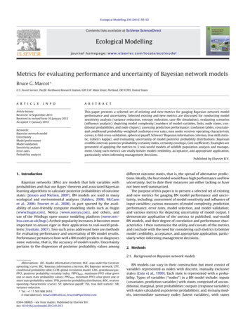
B.G. Marcot / Ecological Modelling 230 (2012) 50–62Bayesian credible intervals, a posterior probability certainty indexand certainty envelope, and a new adaptation of the Gini coefficientand Lorenz curve to depict inequality of PPDs.2.5.1. Bayesian credible intervalsOne existing approach to denoting uncertainty in PPDs is useof Bayesian credible intervals (Bolstad, 2007; Curran, 2005), whichare very loosely an analogue to confidence intervals in frequentist statistics (in some literature, they are confusingly referred toas Bayesian confidence intervals). An X% Bayesian credible intervalof some PPD of an ordinal or continuous scale variable (but not acategorical variable) refers to state-wise probabilities when X/2% isexcluded from the lowest and highest outcome states. Put anotherway, it is the interval determined for the expected value over replicate calculations based on uncertainty distributions of the inputvariables, not for the PPD of a given instance of input values. ABayesian credible interval represents the PPD at a specified levelof acceptability, and in this way differs from a probability densityfunction (and from a frequentist confidence interval).One must decide what credible interval value X to use. In practice, it should be twice the probability of the most extreme stateof interest. For example, if a manager would be concerned oversome extreme outcome, such as a species’ extinction, if there wasa 5% probability or greater of it occurring, then they should notuse anything a 90% credible interval, else it might exclude suchan event.2.5.2. Posterior probability certainty indexAnother metric that can be used to evaluate uncertainty of BNmodel outcomes is the posterior probability certainty index (PPCI).This new metric, first presented here, is based on information theory and specifically is an adaptation of the classic evenness indexfrom species diversity theory (Hill, 1973). Evenness has long beenused to measure the relative distribution of species’ abundances ina community. Here, I extend the concept to PPDs which consist ofpi probability values among N number of states, where pi ranges[0,1] andN pi 1.0.PPCI is calculated asN H (1 J ),whereJ H /Hmax,pi Lj Pii 1there exists a specific range of possible values [PPCIMIN , PPCIMAX ],where PPCIMIN is calculated by setting all other N j states to uniform probabilities, and PPCIMAX is calculated by setting only oneother state to the remaining probability and all other states to zero.That is, PPCIMIN is calculated from j i 1Pi L N 1 mi j 1N jand PPCIMAX is calculated from j ln 1 m iN ji Pi L (1 m) ln(1 m)i 1whereln(pi ),0,m H i 1L 2.5.3. Certainty envelopeAn associated new metric is the certainty envelope, which is therange of possible PPCI values given the probability of one or morestates (up to N 2 states; solutions for N 2 states are trivial). Aspecific PPCI value calculated from a known PPD for a given scenario can then be compared to the certainty envelope to determinethe relative degree of certainty of that outcome to the range of possible values. The certainty envelope is variable because the possiblerange of PPCI values varies as a function of the probability valuesof given states, and only achieves values of 0 and 1 under specialcircumstances of uniform posterior probability distributions andwhen a single state achieves a probability of 1.0, respectively. Otherwise, PPCI can be scaled to the more constrained range of valuescalculated as the certainty envelope.The certainty envelope has utility in some applications wherethe probability of only a subset of outcome states is fixed or known,where others might be more fluid or unknown, and where the manager would want to know the certainty of the PPD given just theknown outcome states. For example, if a BN model is structuredwith five different population levels of a wildlife species (possibleoutcome states), and a particular model run results in predictingprobabilities of the two lowest levels, the manager may wish toknow the overall degree of certainty of the PPD given that particular outcome. That is, how clumped are probability values asdistributed among the outcome states? The less they are evenlydistributed, given a particular result for specific outcome states,the more certain can the manager be of overall model results.The PPCI certainty envelope for a PPD with N states is calculatedas follows. For a given state or set of j states, 1 j (N 2), andtheir known, marginal (summed) posterior probability value(s)H i 153pi 0,pi 0 ln(N). J normalizes the metric proportional to N, so thatand Hmaxthe degree of certainty of PPDs can be compared among outcomeswith different numbers of states N.In information theory, J is a measure of entropy or uncertainty.In the context of risk management, however, one would hope forthe most uneven PPD, that is, an outcome that most clearly suggestsa particular state with the highest probability. Thus, PPCI ranges[0,1] with higher values denoting greater certainty (greater loading of outcome probabilities into fewer outcome states). Modelswith higher PPCI values of their PPDs denote greater certainty inoutcome predictions. Since PPCI is normalized, it can be comparedamong different models with different numbers of outcome states.where L is defined above. Thus, for a given PPD with aspecified probability of a given state or set of j states,PPCIMIN [PPCI P(j)] PPCIMAX . For instance, with N 5 stateswhere the probability of one state j is known, the raw(non-normalized) certainty envelope results in concave upwarddistributions of PPCIMIN and PPCIMAX with convergence at 1.0(Fig. 1). The PPCIMIN curve increasingly skews to the right withgreater number of states.To best compare PPCI values among competing models particularly with different total numbers of states N or different numbersof specified state values j, the range [PPCIMIN , PPCIMAX ] can itselfbe normalized to [0,1], and the relative position of a given valueof [PPCI P(j)] within this range can be calculated by simple linearinterpolation. Thus, the interpolated value of [PPCI P(j)] representsthe proportion (or percentage) of total possible certainty for a givenoutcome state(s) j. This could be valuable information for a managerfaced with only one piece of information, such as the probability of

54B.G. Marcot / Ecological Modelling 230 (2012) 50–62Fig. 1. Non-normalized certainty envelope of a probability distribution with N 5 states across the full range of probability values of a single state, P(NS ).extinction of a species, who might also wish to know the level ofcertainty of the rest of the distribution, i.e., the general dispersionof probabilities among the remaining states.2.5.4. Inequality of posterior probability distributionsAnother new measure of the dispersion of PPD values can makeuse of what is known as the Gini coefficient used in econometrics todepict geographic and social distribution of wealth and resources(Atkinson, 1970; Sadras and Bongiovanni, 2004). The Gini coefficient varies in the range [0,1], and if applied to PPDs in BN models,a value of 0 represents a uniform probability distribution (completeuncertainty) and 1 represents a distribution with one state at 100%probability and all other states at 0% (complete certainty).The Gini coefficient is calculated as the area under the Lorenzcurve, which, applied to BN modeling, is the cumulative probabilityamong outcome states rank-ordered by decreasing values of theirindividual probabilities. Lorenz curves have been used in ecologyto represent the distribution of species abundance proportions inecological communities (Ricotta and Avena, 2002). Applied hereto BN modeling, the Lorenz curve plots cumulative proportion ofposterior states as a function of cumulative probability of posteriorstates, anchored to the (0,0) plot origin.For example, say there is a PPD among 4 outcome states withthe respective probability vector [0.10, 0.85, 0, 0.05]. The vector isfirst reordered in decreasing values, viz., [0.85, 0.10, 0.05, 0], andthen the respective cumulative frequency distribution is calculatedas [0.85, 0.95, 1, 1]. To account for the origin anchor, an initial zerois inserted as [0, 0.85, 0.95, 1, 1], constituting x-axis values. Corresponding y-axis values are merely the increasing proportion of thenumber of states beginning with 0; for our 4-state example here,those values become [0, 0.25, 0.50, 0.75, 1]. Because PPDs in BNmodels sum to 1, associated Lorenz curves always span the domain[0,1].The Lorenz curve plot also includes a positive diagonal line,here spanning (0,0) to (1,1); this is called the line of perfect evenness in econometric literature, and here represents the line of totaluncertainty or highest entropy, that is, the line formed from a uniform probability distribution. The Gini coefficient then is calculatedas the area subtended between the Lorenz curve and the line oftotal uncertainty (perfect evenness). One great advantage of usingthe Gini coefficient as a measure of the dispersion of posteriorprobabilities is that values derived from different models with different numbers of outcome states can be directly compared becauseLorenz curves derived from PPDs always span [0,1].However, one final correction needs to be applied for use in BNmodels. Because BN variables are usually discretized into a finitenumber of mutually exclusive states, the maximum value of thearea within the Lorenz curve – doubled, so that the resulting Ginicoefficient theoretically falls in [0,1] – for n states is 1 (1/n), andasymptotically, limn (2 area) 1.0 (Fig. 2). E.g., if an outcomenode has N 4 discrete states, the maximum value of 2*area 0.75.This maximum area value can be used as a normalizing constant,that is, by dividing the observed area by this correction factor. Then,the resulting adjusted Gini coefficient values can be directly compared among models with different numbers of outcome states.Because of the asymptotic nature of the correction curve, the actualGini values will range [0,1). Exact and approximate calculationsof the Gini coefficient with discrete BN model outcome states arepresented in Appendix A.Fig. 2. Maximum value of the area within the Lorenz curve ( Gini coefficient, heredoubled) increases asymptotically to 1.0 as a function of the number of states, asapplied to posterior probabilities from Bayesian network models.

B.G. Marcot / Ecological Modelling 230 (2

2.4. Metrics of BN model prediction performance Several metrics can be used to evaluate the performance of BN models when cases are available for which outcomes are known. Existing metrics useful to BN modeling include use of confusion tables, receiver operating characteristic curves, k-fold cross-validation, and performance indices such as .