Transcription
Research ArticleJOURNAL OF COMPUTATIONAL BIOLOGYVolume 27, Number 0, 2020# Mary Ann Liebert, Inc.Pp. 1–13DOI: 10.1089/cmb.2019.0265Solution of Ion Channel Flow Using ImmersedBoundary–Lattice Boltzmann MethodsDownloaded by National Taiwan University N.T.U. Package from www.liebertpub.com at 12/22/19. For personal use only.KUMAR SAURABH,1,2 MAXIM SOLOVCHUK,2 and TONY WEN HANN SHEU1ABSTRACTPoisson–Nernst–Planck (PNP) model has been extensively used for the study of channel flowunder the influence of electrochemical gradients. PNP theory is a continuum description ofion flow where ionic distributions are described in terms of concentrations. Nonionic interparticle interactions are not considered in this theory as in continuum framework, theirimpact on the solution is minimal. This theory holds true for dilute flows or flows wherechannel radius is significantly larger than ion radius. However, for ion channel flows, wherechannel dimensions and ionic radius are of similar magnitude, nonionic interactions, particularly related to the size of the ions (steric effect), play an important role in defining theselectivity of the channel, concentration distribution of ionic species, and current across thechannel, etc. To account for the effect of size of ions, several modifications to PNP equationshave been proposed. One such approach is the introduction of Lennard-Jones potential tothe energy variational formulation of PNP system. This study focuses on understanding therole of steric effect on flow properties. To discretize the system, Lattice Boltzmann methodhas been used. The system is defined by modified PNP equations where the steric effect isdescribed by Lennard-Jones potential. In addition, boundary conditions for the complexchannel geometry have been treated using immersed boundary method.Keywords: immersed boundary method, ion-channel flow, Lattice Boltzmann method, steric effect.1. INTRODUCTIONransfer of bioions (Na , K , Ca2 , and Cl-) across the cell membrane is one of the most fundamentalphysiological processes. Bioion transport results in the generation and propagation of action potential inthe neurons (Colbert and Pan, 2002), muscle contraction (Kuo and Ehrlich, 2015), conversion of light toelectric signals in photoreceptors, and so on. Several specialized structures have evolved to ensure themovement of ions across the membrane and ion channels form a subset of these structures. Ion channels areembedded across the cell membrane and constitute a hydrophilic environment. Theoretical study of ionchannels can be segregated into three different categories: (1) closing and opening of the ion channels (gatingmechanism), (2) selectivity of ions, and (3) permeability.Based on their gating mechanisms, ion channels can be broadly categorized into voltage-gated, ligandgated (neurotransmitter), and lipid-gated channels. Other gating mechanisms such as the ones found inT1Department of Engineering Science and Ocean Engineering, National Taiwan University, Taipei, Taiwan.Institute of Biomedical Engineering and Nanomedicine, National Health Research Institute, Zhunan, Taiwan.21
Downloaded by National Taiwan University N.T.U. Package from www.liebertpub.com at 12/22/19. For personal use only.2SAURABH ET AL.mechanosensitive channels and light-gated channels are also present. This study is focused on exploring thedependence of selectivity of channel on size of the ions.In biological simulations, ion channels have been studied using continuum models based on Poisson–Nernst–Planck (PNP) equations, Monte Carlo method, Brownian dynamics, and molecular dynamics.Continuum-based approaches have often been deemed inaccurate, when compared with other approaches, dueto their simplified approximations of atomic properties of the channel and the solution (Sagui and Darden,1999; Corry et al., 2000; Im and Roux, 2002). In contrast, continuum models have been shown to be moreefficient in studying the averaged properties of the system.Over the years, several modifications to the standard PNP equations have been proposed in the literatureto counter the shortcomings of PNP model (Gillespie, 2008; Liu, 2009; Kurnikova et al., 1999; Eisenberg,2010). Liu and his group (Sheng et al., 2008; Liu, 2009; Xu et al., 2012) pioneered energetic variational(EnVar) approach that describes the energy of the system as Helmholtz free energy of classical thermodynamics (Sagui and Darden, 1999). This enabled the inclusion of multi-physics models in traditional PNPsystem. Kurnikova with her group (Kurnikova et al., 1999; Graf et al., 2004; Kurnikova and Coalson, 2005)tackled the problem by resorting to density functional theory. Nonner and Eisenberg (1998), Nonner et al.(1998, 2000), and Boda et al. (2002) developed a simplified model for ions present in the bulk solution andinside the filter by incorporating the effect of the size of ionic species. In their further research, they successfully showed that selectivity of certain types of ion channels can be explained with their model. Thisapproach was further generalized by Eisenberg (2010), Eisenberg et al. (2010a,b, 2011), Hyon et al. (2011),Mori et al. (2011), and Horng et al. (2012) by adopting the EnVar approach. A detailed review of thesemathematical models can be found in Chen and Wei (2016). In this study, we follow the methodology proposedin Horng et al. (2012). However, we are performing a 2D analysis as opposed to 1D analysis performed therein.In this study, we solve for a 2D ion-channel flow using Lattice Boltzmann method (LBM). To addresscomplex channel geometry, immersed boundary method (IBM) has been used ensuring the proper implementation of boundary conditions. The outline of the article is as follows. Basic mathematical model forstandard and modified PNP equations is covered in Section 2. Furthermore, a brief introduction of LBM, inthe context of PNP equations has also been provided. In Section 3, methodology to implement IBM for noflux boundary conditions, with regard to Nernst–Planck equation, is discussed. Section 4 covers numericalvalidation of the scheme. Conclusion is provided in Section 5.2. MATHEMATICAL MODELS2.1. PNP equationThe PNP model is a well-established model for the study of ion transport. The model is constituted by- :( /) q0 NXzi eci(1a)i 1@ci :Ji 0‚@tJi - Di ( ci i 1‚ . . . :‚ Nzi eci /)‚KB T(1b)(1c)where e is the dielectric constant, / is the electrostatic potential, and q0 is the fixed charge density. PoissonEquation (1a) describes the electrostatic potential field for the provided charge distributions. As for theNernst–Planck Equation (1b), it describes the evolution of concentration of ionic species under the influence of electrochemical gradient. In Equation (1c), ci represents the concentration, Ji represents the ionicflux, Di represents diffusivity, zi represents valency, e is the elementary charge, KB is the Boltzmannconstant, and T is the temperature. Please note that subscript ‘‘i’’ stands for the ith ionic species. Inclusionof steric effect results in the modification of the flux term in the NP equation.Ji - Di ( ci NXzi eci / cigij cj )‚KB Tj 1(2)where gij are the coefficients dependent on the size of the constituent ions. A detailed derivation can befound in Horng et al. (2012) and the references therein.
SOLUTION OF ION CHANNEL FLOW USING IBM–LBM32.2. Lattice Boltzmann methodLBM is derived from the mesoscopic description of flow based on kinetic theory. In this study, instead ofsolving PNP, we essentially solve N 1 Boltzmann equations, one for Poisson equation, whereas the restrepresenting N Nernst–Planck equations. Boltzmann equation is given by@f@f e O(f )‚@t@x(3)where f is the density distribution function, e is the lattice velocity, and O(f) is the collision operator. Upondiscretization, Equation (3) can be rewritten asDownloaded by National Taiwan University N.T.U. Package from www.liebertpub.com at 12/22/19. For personal use only.fa (x ea Dt‚ t Dt) fa (x‚ t) DtO(f (x‚ t)):(4)The collision operator can be approximated by Bhatnagar-Gross-Krook (BGK) operator (Bhatnagaret al., 1954) and Equation (4) can be simplified tofa (x ea Dt‚ t Dt) fa (x‚ t) 1 eq(f (x‚ t) - fa (x‚ t)):s a(5)In this study, a represents the lattice direction and s is the relaxation parameter. For this study we areconsidering a D2Q9 lattice, that is, a 0, ., 8.For Poisson equation, the equivalence between mesoscopic and macroscopic properties is establishedthrough the following relations:X/ faP(6a)afaeq wa /:Similarly, defining a set of distribution functions for ion concentration such thatXci fa‚NPi(6b)(7a)afa‚eqi wa ci (1 ea :Veff)c2s(7b)lead to Nernst–Planck equations, where cs represents the velocity of sound and Veff - Di KzBi eT /.2.3. Geometry and boundary conditionsFor this study, we are considering the same geometry as in Horng et al. (2012). The channel Schematically shown in Figure 1 is 50 Å long and the width varies with the channel length. The maximum widthhas been taken as 80 Å and the filter region lies between 20 and 30 Å along the channel axis.Radius of the channel varies as a function given byr(z) rmax - rmin(z -a 2p) rmin ‚2(8)(a 2)where z is the location in the axial direction, r(z) is the radius of channel at z, rmax 40 Å, rmin 3.5 Å,a 50 Å, p 4, and width 2r(z).The system is represented by Equation (5), whereas the equilibrium distribution function is represented byEquations (6b) and (7b) for Poisson and Nernst–Planck equations, respectively. To obtain the dimensionlessform of the governing equations, we adopt the following nondimensionalization parameters:ci/Vcei ‚V ‚/ KB t eKB TcNa‚ maxstei Di t 2 s ‚‚DLrefDNaLref DNaLref rmin2pFor this study, bulk concentration is assumed to be constant. This assumption will lead to constant ci andby extension, constant / boundary conditions at the left, and right ends of the channel.
4SAURABH ET AL./(0) /0 (0);ci‚ t (0) ci‚ 0 (0);/(L) /0 (L)(10a)ci‚ t (L) ci‚ 0 (L) 2 -(10b)0.5-Please note that we are considering four ionic species Na , Ca , Cl , and CO . In Equation (10b), ‘‘i’’represents Na , Ca2 , and Cl- as they are distributed in the whole domain. Since CO0.5- is confined to thefilter region, CO0.5- must satisfy the no-flux condition at the boundary of the filter. To confine CO0.5- insidethe filter, we introduce a restricting potential that can be expressed asV Vmax c(z - 0:5l)2 ‚Downloaded by National Taiwan University N.T.U. Package from www.liebertpub.com at 12/22/19. For personal use only.where c is defined in a way that V Vmax on either end of the filter. This further leads to the modification ofNernst–Planck equation for CO0.5Ji - Di ( ci zi ecici / V):KB TKB TBoundary conditions are shown in Figure 2.For LBM, we transform the boundary conditions in terms of distribution functions.faP (0) 2wa /0 (0) - f -P a (0);fi‚NPa (0) 2wa ci‚ 0 (0) - fi‚NP- a (0);faP (0) 2wa /0 (L) - f -P a (L)(11a)fi‚NPa (L) 2wa ci‚ 0 (L) - fi‚NP- a (L):(11b)a is the direction of the unknown component of distribution function, whereas -a is the opposite direction.At the channel–membrane interface, Neumann boundary condition for Poisson equation and no-fluxboundary condition for Nernst–Planck equations have to be satisfied. In Poisson equation, for the implementation of jump condition at membrane–channel interface, matched interface, and boundary method(Zhu et al., 2006; Pan et al., 2010; Zheng and Wei, 2011) has been used, whereas for no-flux boundarycondition in Nernst–Planck equation, a methodology falling within the immersed boundary framework hasbeen used. Details of its implementation are discussed next.2.3.1. Immersed boundary method. IBM was developed by Peskin (1977) for the simulation ofblood flow in heart. Since then, there have been a number of refinements and modifications. A detailedreview can be found in Mittal and Iaccarino (2005). In this study, for a proper implementation of no-fluxboundary condition for the Nernst–Planck equation we follow the methodology proposed in Shu et al.(2013). The boundary conditions are given as( cBi zi cBi /B ):n 0( cBi zi cBi /B NXj 1FIG. 1.Schematic of the channel.standard PNPcBi gij cBj ):n 0modified PNP‚(12a)(12b)
SOLUTION OF ION CHANNEL FLOW USING IBM–LBMDownloaded by National Taiwan University N.T.U. Package from www.liebertpub.com at 12/22/19. For personal use only.FIG. 2.5Boundary conditions.where n is the vector normal to the interface. To represent the effect of immersed boundary, we modify theNernst–Planck equations to@ci :Ji f@t1fa (x ea Dt‚ t Dt) fa (x‚ t) (faeq (x‚ t) - fa (x‚ t)) Fa Dt‚s(13a)(13b)where f represents the forcing term due to the presence of immersed boundary. To calculate the forcingterm, fractional step methodology has been implemented. To illustrate implementation steps, we are usingstandard PNP as an example. Extension to PNP-steric equation is straight forward. For the predictor stepEquation (1b) can be solved using LBM to obtain the intermediate concentration value represented by c i .This process can be represented asCollision step: fa (x‚ t) fa (x‚ t) 1s (faeq (x‚ t) - fa (x‚ t))Streaming step: fa (x ci Dt‚ t ) fa (x‚P t) Flow variable calculation: c (x) ia fa (x‚ t ). Next we calculate normal flux at the boundary, Equation (12a). To obtain normal flux, we have tocalculate intermediate concentration and gradients of intermediate concentration and potential at theboundary. We use delta function for their calculation. The process can be represented as@c i (x) ci ‚ j 1‚ k - ci ‚ j - 1‚ k ;@x2Dx@c i (x) ci ‚ j‚ k 1 - ci ‚ j‚ k - 1 @y2Dy@/(x) / j 1‚ k - / j - 1‚ k@/(x) / j‚ k - 1 - / j‚ k - 1 ;@x@y2Dx2Dy 4 X@ci (x) @ci (x)B dBxi c ‚i@x@yx 1 4X@/(x) @/(x) /B dBxi@x@yx 1Bc ‚ i4XdBx c i (x)x 1Delta function is calculated as( - xi j- yi j1 - jyBDy‚1 - jxBDxdBxi 0‚otherwiseif jxB - xi j Dx and jyB - yi j Dy1, 2, 3, and 4 are the neighboring points such that jxB-xij Dx and jyB-yij Dy for i 1, ., 4. Neighboringpoints corresponding to boundary point B are labeled clearly in Figure 3.
6SAURABH ET AL.Downloaded by National Taiwan University N.T.U. Package from www.liebertpub.com at 12/22/19. For personal use only.FIG. 3. A generalized schematic of membrane–channel interface. 1, 2, 3, and 4 representthe neighboring nodes, whereas B represents theboundary node.BB ‚ BOnce we obtain the values of c ‚i ‚ ci , and V/ , we can calculate the normal flux at the boundaryBBBfl ( ci zi ci / ):n. In the corrector step, we assign a forcing term at the boundary such that the no-fluxboundary condition is satisfied. This results in forcing term -flB. Then we extrapolate this value to theneighboring nodes using delta function. In LBM frame the process can be described asBCollision: fa (x‚ t ) fa (x‚ t ) 1s (faeq (x‚ t ) - fa (x‚ t )) Fa (x‚ t)Dt Streaming: fa (x ci Dt‚ t Dt) f (x‚ t )aPBwhere Fa ðx; tÞ ¼ - j;k dBjk fl . 3. NUMERICAL VALIDATIONIn this study, we have analyzed the effect of steric term on the concentration distribution of ionic speciesin the channel. This analysis is an extension of the analysis performed in Horng et al. (2012) where theequations were solved in an axis-symmetric 1D framework. To validate our results, we have compared theconcentration profiles along channel axis with their results and a significant match has been observed. Forall the cases, we have fixed the potential as 100 mV on either side of the channel. Concentration of Na ionis fixed at 100 mM on either side, whereas concentration of Ca2 ion varies. Cl- is kept at a concentration tomake the bulk solution electrically neutral. CO0.5- concentration acquires the value equivalent to fourcarboxyl groups and it is distributed uniformly inside the filter. The maximum value of nondimensionalizedrestricting potential is kept at 200. Diffusion coefficients (m2/s) in bulk solution are DNa 1.334 · 10-9,DCa 0.792 · 10-9, DCl 2.032 · 10-9, and DCO 0.76 · 10-9. In the filter region, diffusion coefficients areset to 1/20th of their bulk values. Dielectric constant is 80 0 in the bulk solution, whereas it takes a value of30 0 inside the filter. In membrane region, we assign it a value of 2 0.In the first case, we are reporting the impact of increasing the steric effect on the centreline concentrationprofile. The coefficient values are listed in Table 1. Concentration of Ca2 is fixed at 1 · 10-3 M on eitherside of the channel.Table 1. Different Set of Coefficientsof Steric TermsgNaNagNaCagNaOgCaCagCaOgOO00000010-46.41 · 10-58.19 · 10-41.64 · 10-41.00 · 10-31.64 · 10-210-26.41 · 10-38.19 · 10-21.64 · 10-21.00 · 10-11.64
7In PNP-steric equations, we model electrochemical and steric forces acting on ionic species. Electrochemical forces originate from ionic interactions and potential gradient. Depending upon the nature ofinteracting species, electrochemical forces could be attractive or repulsive in nature. Steric forces representnonionic interactions and are typically repulsive for small distances. Thus, we have considered only therepulsive part of nonionic interactions in our model. In the absence of steric forces, one would expect that Na and Ca2 ions present in the bath, to get attracted toward anionic filter repelling each other at the same time,whereas Cl- to be pushed away from the filter. Owing to high concentration of CO0.5- inside the filter, theseinteractions would result in the accumulation of cationic species inside the filter. This can be observed clearlyin Figure 4a. Thus, for this study, accumulation of cationic species in the filter is a typical result of standardPNP model. Please note that an accumulation of carboxyl group toward the centre is significantly influencedby restricting potential and different restricting potential profiles will result in different concentration profiles.Next we studied the impact of adding steric forces to the system. It is important to note that the ratio ofsteric terms for species is fixed; however, their absolute value is not. Thus, we have considered threedifferent sets of values as shown in Table 1. Steric forces would introduce more repulsion, which wouldoppose the accumulation of ionic species inside the filter. As a result, maximum concentration inside thechannel would drop and the profile would become flatter. The same behavior can be observed uponcomparing Figure 4a and b, where Figure 4a is a solution of standard PNP. Owing to their different valency,Ca2 experiences higher attraction toward the filter compared with Na . For sufficiently large steric coefficient values, repulsion forces for Na could overcome the attraction forces and Na ions would bepushed away from the centre of the filter toward the corners. This would result in creation of a depletionzone in the centre of the filter and accumulation toward the corners. The concentration profile that showed asingle peak for previous cases will show two peaks near the corners. This is termed as the splitting ofconcentration profile. As expected, Ca2 experiences further flattening of the concentration profile; however, concentration profile does not split. In Figure 4c, where gNaNa 10-2, we can clearly observe thisbehavior.concentration in Ma30025020015010050010OX2NaCaCl152025303540z in angstromconcentration in Mb80OX260Na40Ca20010Cl152025303540z in angstromcconcentration in MDownloaded by National Taiwan University N.T.U. Package from www.liebertpub.com at 12/22/19. For personal use only.SOLUTION OF ION CHANNEL FLOW USING IBM–LBM20OX215Na10Ca5010Cl152025303540z in angstromFIG. 4. Species concentration distributions for various gNaNa. Vmax 200, /0 /L 100 mV and Na0 NaL 100mM, Ca20 Ca2L 1 mM. (a) gNaNa 0, (b) gNaNa 10-4, and (c) gNaNa 10-2. The results are in good agreement withthe results published in Horng et al. (2012).
Downloaded by National Taiwan University N.T.U. Package from www.liebertpub.com at 12/22/19. For personal use only.8SAURABH ET AL.Figure 5 illustrates the impact of increasing the concentration of Ca2 ion while keeping the concentrationof Na at a fixed value in the absence of steric force. As the concentration of Ca2 in the bath increases, moreand more Ca2 ions get accumulated inside the filter and the concentration profile adopts a Maxwelliandistribution. It should be noted that in biological systems, Ca2 concentration varies over a range of 1 · 10-8 to1 · 10-2 M. Therefore, the bath concentration is a representative of realistic scenario. Although accumulationof Ca2 increases with the increasing bath concentration, only at the moment when Ca2 bath concentrationreaches 10-4 M value, ionic concentration of both cationic species is comparable inside the filter.Next, we introduced steric forces where gNaNa 1 · 10 - 2 and performed simulation for the same set ofparameters and bulk concentrations. The results are illustrated in Figure 6.In this study, we observe a significant drop in the concentrations of all species in the filter. As theconcentration of Ca2 in the bath increases, more Ca2 are getting accumulated inside the filter, whichincrease both electrostatic and steric repulsions for Na . As a result, with increasing Ca2 , we observe higherdepletion in the concentration profile of Na ion in Figure 6. Similar to the previous case Figure 5, an increasein bath concentration leads to an increase in the concentration inside the filter. However, the concentrations ofboth the species become comparable for a much smaller Ca2 bath concentration. This can be observedclearly from the binding curves shown in Figure 7 where binding ratio for calcium is defined asBinding ratio No:Ca2 No: Ca2 ions inside filter:ions inside filter No: Na ions inside filterSignificant difference between the binding curves with and without steric term highlights the limitationof standard PNP model. Steric term greatly enhances the selectivity of Ca2 ions. In addition, the bindingcurves match significantly with the ones published in Horng et al. (2012).FIG. 5. Species concentration distributions at fixed Na bath concentration of 0.1 M and different Ca2 bath concentrations. Vmax 200, /0 /L 100 mV, and gNaNa 0. (a) Ca2 1 · 10--7 M, (b) Ca2 1 · 10--6 M, (c) Ca2 1· 10-5 M, (d) Ca2 1 · 10-4 M, (e) Ca2 1 · 10-3 M, and (f) Ca2 1 · 10-2 M. The results are in good agreementwith the results published in Horng et al. (2012).
10.8Binding ratioDownloaded by National Taiwan University N.T.U. Package from www.liebertpub.com at 12/22/19. For personal use only.FIG. 6. Species concentration distributions at fixed Na bath concentration of 0.1 M and different Ca2 bath concentrations. Vmax 200, /0 /L 100 mV, and gNaNa 0.01. (a) Ca20 Ca2L 10-7 M, (b) Ca20 Ca2L 10-6 M, (c)Ca20 Ca2L 10-5 M, (d) Ca20 Ca2L 10-4 M, (e) Ca20 Ca2L 10-3 M, and (f) Ca20 Ca2L 10-2 M. The resultsare in good agreement with the results published in Horng et al. (2012).0.6 Na with steric effect2 Cawith steric effect Na without steric effect0.42 Cawithout steric effect0.2010-710-610-510-410-310-2CaCl (in M) added to 0.1 M NaCl2FIG. 7.The predicted binding curves with (gNaNa 0.01) and without (gNaNa 0) steric forces.9
10SAURABH ET AL.a50concentration in MNa40CaCl3020100-10-50510bconcentration in MDownloaded by National Taiwan University N.T.U. Package from www.liebertpub.com at 12/22/19. For personal use only.x in angstrom8NaCa6Cl420-10-50510x in angstromFigure.8FIG. 8. Species concentration distributions in the direction perpendicular to the channel axis. Vmax 200,/0 /L 100 mV and Na0 NaL 100 mM, Ca20 Ca2L 1 mM. (a) gNaNa 0 and (b) gNaNa 10-2.To understand the effect of two dimensionality of the system we have plotted the concentration profilesin the direction perpendicular to the channel axis at half length of the channel. In Figure 8, in the absence ofsteric effect, we observe that the maximum concentration lies at centre of the channel, which is coincidentwith the channel axis, whereas at the channel–membrane interface the concentration is zero. As wasobserved along the channel axis, steric effect will oppose the accumulation of ionic species, pushing themtoward the channel–membrane interface. As before, this would result in flattening of the concentrationprofile, this time along the direction of channel width. For gNaNa 0.01, we observed splitting in concentration profile of Na ion thereby establishing two peaks near the channel–membrane interface.So far we have discussed the role of steric repulsion in determining the ionic concentration distribution.Another factor that can significantly influence ionic distribution is the geometry of the channel. To illustratethis further, we are considering the channel where the selectivity filter is not cylindrical. Channel geometryis given in Figure 9. To avoid any influence from the steric repulsions, we are considering gNaNa 0. Theresults are plotted in Figure 10. Upon comparison with the previous nonsteric case, we observed an overallincrease in the concentration of CO0.5-. Thus, as the concentration of Ca2 in the bath increases, higherconcentration of Ca2 will get accumulated at the centre of the filter. This will result in the channelbecoming Ca2 selective for a lower Ca2 bath concentration. As the only difference between the currentand the previous channel is the shape of the filter region, this increase must be an outcome of the reductionof minimum channel width.4. CONCLUSIONIn this article, we performed a 2D analysis of ion channel using EnVar approach-based PNP models. Thesystem was descretized using LBM. For the complex boundary, we used no-flux boundary conditionenforced IBM. There is a good match between our results and the ones available in literature. One of thekey features of the steric term is to provide repulsion mechanism among ionic species that should eventually result in a splitting of concentration profile leading to the emergence of peaks in concentration near
SOLUTION OF ION CHANNEL FLOW USING IBM–LBMDownloaded by National Taiwan University N.T.U. Package from www.liebertpub.com at 12/22/19. For personal use only.FIG. 9.11Schematic of the new channel.the corners of the filter and channel–membrane interface. In addition, we have successfully illustrated thatfilter geometry can significantly influence concentration profile.Conclusively, steric repulsions and filter geometry play significant roles in defining the ionic distributioninside the channel. Thus, to obtain more accurate results for ion flows, it is very important to correctlydefine the coefficients for the steric term and to construct channel geometry more accurately. Furthermore,it is important to note that modified PNP-based analysis has been successful at replicating results based onnoncontinuum models and is computationally inexpensive compared with its counterparts. Thus, it isFIG. 10. Species concentration distributions for the cases at the fixed Na bath concentration of 0.1 M under variousCa2 bath concentration. (a) Ca2 1 · 10-7 M, (b) Ca2 1 · 10-6 M, (c) Ca2 1 · 10-5 M, (d) Ca2 1 · 10-4 M, (e)Ca2 1 · 10-3 M, and (f) Ca2 1 · 10-2 M.
12SAURABH ET AL.worthwhile to investigate it further to make it more robust. To the best of authors’ knowledge, this is thefirst time PNP-steric model, based on EnVaR approach, has been solved using LBM–IBM for a 2D ionchannel.AUTHOR DISCLOSURE STATEMENTThe authors declare they have no competing financial interests.Downloaded by National Taiwan University N.T.U. Package from www.liebertpub.com at 12/22/19. For personal use only.FUNDING INFORMATIONThis study was supported in part by NHRI (National Health Research Institute, Institute of BiomedicalEngineering and Nanomedicine, Zhunan, Taiwan, Project number BN-106-PP-08) and MOST (Ministry ofScience and Technology, Taipei, Project number MOST-106-2115-M-400-001-) project.REFERENCESBhatnagar, P.L., Gross, E.P., and Krook, M. 1954. A model for collision processes in gases. I. Small amplitudeprocesses in charged and neutral one-component systems. Phys. Rev. 94, 511–525.Boda, D., Busath, D., Nonner, W., et al. 2002. Monte Carlo simulations of ion selectivity in a biological Na channel:Charge–space competition. Phys. Chem. Chem. Phys. 4, 5154–5160.Chen, D., and Wei, G.-W. 2016. A review of mathematical modeling, simulation and analysis of membrane channelcharge transport. arXiv:1611.04573v1.Colbert, C., and Pan, E. 2002. Ion channel properties underlying axonal action potential initiation in pyramid neuron.Nat. Neurosci. 5, 533–538.Corry, B., Kuyucak, S., and Chung, S.H. 2000. Tests of continuum theories as models of ion channels. II. Poisson–Nernst–Planck theory versus Brownian dynamics. Biophys. J. 78, 2364–2381.Eisenberg, B. 2010. Multiple scales in the simulation of ion channels and proteins. J. Phys. Chem. C 114, 20719–20733.Eisenberg, B., Hyon, Y., and Liu, C. 2010a. Energy variational analysis of ions in water and channels: Field theory forprimitive models of complex ionic fluids. J. Chem. Phys. 133, 104104.Eisenberg, B., Hyon, Y., and Liu, C. 2011. A mathematical model for the hard sphere repulsion in ionic solutions.Commun. Math. Sci. 9dd, 459–475.Eisenberg, R.S., Hyon, Y., and Liu, C. 2010b. Energetic variational analysis EnVarA of ions in calcium and sodiumchannels. Biophys. J. 98, 515a.Gillespie, D. 2008. Energetics of divalent selectivity in a calcium channel: The ryanodine receptor case study. Biophys.J. 94, 1169–1184.Graf, P., Kurnikova, M.G., et al. 2004. Comparison of dynamic lattice Monte Carlo simulations and the dielectric selfenergy Poisson-Nernst-Planck continuum theory for model ion channels. J. Phys. Chem. 108, 2006–2015.Horng, T.L., Lin, T.C., Liu, C., et al. 2012. PNP equation with steric effects: A model of ion flow thr
For this study, we are considering the same geometry as in Horng et al. (2012). The channel Schema-tically shown in Figure 1 is 50 A long and the width varies with the channel length. The maximum width has been taken as 80 A and the filter region lies between 20 and 30 A along the channel axis. Radius of the channel varies as a function .