Transcription
Compressing Network GraphsAnna C. GilbertAT&T Labs-Research180 Park AvenueFlorham Park, NJ 07932Kirill Levchenko University of California, San Diego9500 Gilman Drive Dept 0114La Jolla CA d.eduABSTRACTGraphs form the foundation of many real-world datasetsranging from Internet connectivity to social networks. Yetdespite this underlying structure, the size of these datasetspresents a nearly insurmountable obstacle to understandingthe essential character of the data. We want to understand“what the graph looks like;” we want to know which vertices and edges are important and what are the significantfeatures in the graph. For a communication network, suchan understanding entails recognizing the overall design ofthe network (e.g., hub-and-spoke, mesh, backbone), as wellas identifying the “important” nodes and links.We define several compression schemes, including vertexsimilarity measures and vertex ranking. We present a system for condensing large graphs using both auxiliary information (such as geographic location and link type in thecase of communication networks), as well as purely topological information. We examine the properties of these compression schemes, demonstrate their effects on visualization,and explore what structural graph properties they preservewhen applied to both synthetic and real-world networks.1.INTRODUCTIONMassive graphs are everywhere, from social and communication networks to the World Wide Web. The geometricrepresentation of the graph structure imposed on these datasets provides a powerful aid to visualizing and understandingthe data. However even with this aid, these graphs are toolarge to comprehend without additional processing. In thispaper, we consider creating graphical summaries of the largegraphs arising in the domain of enterprise IP networks. Ourmethods do not limit us to this domain; rather, this domainis rich in large highly engineered graphs.We do this by transforming the original graph into a smallerone using structural features of the graph that have wellunderstood semantics in our domain. The resulting smaller, A significant portion of this work was done while KirillLevchenko was visiting AT&T Labs–Research.Permission to make digital or hard copies of all or part of this work forpersonal or classroom use is granted without fee provided that copies arenot made or distributed for profit or commercial advantage and that copiesbear this notice and the full citation on the first page. To copy otherwise, torepublish, to post on servers or to redistribute to lists, requires prior specificpermission and/or a fee.Copyright 200X ACM X-XXXXX-XX-X/XX/XX . 5.00.and usually annotated, graph can then be visualized, and,we hope, understood, by a human being confronted withsuch a dataset. We refer to this process as graph compression, or, more properly, semantic graph compression,to distinguish it from algorithmic graph compression wherea graph is compressed in order to reduce the time or spacecomplexity of a graph algorithm.We define two categories of compression schemes, onebased on the notion of vertex importance and another on thenotion of vertex similarity, which we describe in Section 3,after discussing related work in the next section (Sec. 2). InSection 4 we experimentally verify our results on two synthetic and four real-world datasets, using Arc [6], a graphcompression tool expressly developed for this purpose, andwhose description we omit due to space constraints. Finally,Section 5 concludes the paper.2. RELATED WORKAlgorithmic Compression.Previous work in graphcompression has been concerned exclusively with compressing graphs for input to algorithms, where the (smaller) compressed representation preserves some property used by thealgorithm.Feder and Motwani [5] consider transforming a graph intoa smaller one (in terms of the number of vertices and edges)that preserves certain properties of the original graph, suchas connectivity. A graph compressed in this manner is suitable for (more efficiently) computing certain graph functions, such all-pairs shortest paths. Although our sharedmedium compression scheme has similarities with this work,our goal is to preserve the semantics of the original graph,rather than its algorithmic properties.Adler and Mitzenmacher [1] and Suel and Yuan [12] consider losslessly compressing the Web Graph for efficient searchengine storage and retrieval. Although it differs from ourwork in that only the representation, and not the actualgraph, is compressed, their compression process itself mayreveal semantically-relevant information.The Web Graph.The link structure of the WorldWide Web has seen considerable study in the context ofweb search, an important step of which is ranking the resultsin order of relevance. The most widely studied algorithmsfor this—PageRank [10], HITS [7], and SALSA [9]—use aMarkov model, motivated by the image of a web surfer visiting web pages by following links or jumping to a randompage. Because our graph is undirected, such a process doesnot reveal additional information; however other spectraltechniques, which we did not investigate, may have applica-
tions to our problem.Recently, White and Smyth [14] introduced a number ofnew notions of vertex importance using both paths and random walks. Our paths scheme is a specialization of theirweighted paths algorithms.In [8], Kumar et al. infer certain relationships betweennodes in the Web Graph based on the link structure. (Thesame idea is also found in Kleinberg’s HITS [7], which infers hub-authority relationships between websites.) Our redundant vertex elimination scheme is based on this idea ofrecognizing local structures.IP Network Measurement.Faloutsos et al. in [4]reported on the statistical properties of the autonomous system network graph as well as Internet router graphs. Whiletheir goal is to characterize the statistical properties of thenetwork graph, we are interested in understanding a particular instance of a network. Nonetheless, their work hasled to the emergence of Internet topology generators, oneof which, inet-3.0 [15], was used to generate one of oursynthetic datasets.Spring, Mahajan, and Wetherall in [11] used novel techniques to derive approximate real-world IP topologies. Weuse several of their publicly available datasets in experiments.1Graph Visualization.Our work uses neato, a partof GraphViz [2], which is a publicly available graph visualization tool developed at AT&T Labs–Research. GraphVizalso includes gvpr, a graph processing tool that has some offunctionality of Arc [6], our graph compression tool.3.COMPRESSION SCHEMESWith the application of communication network visualization in mind, let us define a compression scheme to bea transformation of a network graph into a much smaller,possibly annotated, graph that preserves the salient characteristics of the original network. What these might beis, necessarily, an elusive concept; nevertheless we will takethese to be characteristics that have a straightforward, realworld interpretation in the domain of communication networks. One obvious such characteristic is connectivity: if anunderlying network is connected, the compressed networkshould be connected also. Therefore, we shall attempt tojustify our compression schemes based on their real-worldinterpretation.One way to classify compression schemes is into those thatare purely topological, that is, those that rely only on theunderlying network graph, and into those that rely on additional vertex or edge attributes. In an IP network, forexample, vertices (hosts) may be labeled as routers or workstations: for such a network a reasonable compressed representation may be the network graph induced by the setof router vertices. While such a compression scheme is inherently more powerful than a purely topological one, itsrequisite information may not always be available.Orthogonal to the classification above, we have identifiedtwo basic types of compression schemes: those that compress the network based on a notion of node importance,and those based on a notion of similarity. An importancecompression scheme ranks vertices in order of importance(or based on an importance predicate), producing the in1Our affiliation should not be seen as an endorsement of theaccuracy of Rocketfuel data.duced graph as the compressed network. Such compressionschemes are presented in section 3.1. A similarity compression scheme, on the other hand, combines similar verticesinto a single vertex in some manner; these schemes are covered in section 3.2. We let G (V, E) denote the networkgraph G with vertex set V and edge set E in what follows.3.1 Importance Compression SchemesThe notion of a node’s importance in a graph has receivedconsiderable attention in the domain of Web graphs (in thecontext of ranking Web search results), as well as in the domain of social networks. We consider importance to be aweight function on vertices, and describe three such functions: two based on degree and one based on shortest pathsin the graph. We then consider how an importance notioncan be used to compress a graph in Section 3.1.3.3.1.1 Degree-based ImportanceThe degree of a node is arguably one of the simplest andmost intuitive measures of importance in a communicationnetwork. One may reasonably posit that the greater thedegree, the more important the network node, especiallyin view of the preferential attachment interpretation of thepower law phenomenon. There are a number of essentiallyequivalent ways to define such a weight function; let uschoosewdeg (v) {u V : deg(u) deg(v)} / V ,which gives a weight in the range (0, 1].Unfortunately, wdeg tends to favor dense components ofa graph because the weight of a vertex is its relative rankcompared to all the vertices in the graph. For this reason,we developed a localized variant:wbeta (v) {u N(v) : deg(u) β · deg(v)} / N(v) ,where β is a parameter and N(v) is the set of vertices adjacent to v. The Beta weight function assigns weight relative to the neighborhood of a vertex, rather than the wholegraph.3.1.2 Shortest Path-based ImportanceDistance is another fundamental graph property that hasa natural interpretation in the domain of IP networks, andthat is as the number of hops between two routers. It seemsreasonable, then, to consider weight functions based on thisquantity. Recall that the eccentricity of a vertex is definedto be the maximum distance between itself and another vertex. It can be thought of as a measure of how far the vertexis from the “center” of the graph. However because a communication network may not have a meaningful “center,”we did not further pursue such a weight function.Instead, we considered the following weight function. Define the Path weight wpath of a vertex (sometimes also calledits betweenness in social networks) to be the number ofshortest paths between any two (not necessarily distinct)vertices in the graph through the vertex, divided by thesquare of the total number of vertices in the graph; whenthere are multiple shortest paths between a pair of vertices,each is weighted equally so that the sum of the weights of allshortest paths between the two vertices is 1. More formally,defineX {π Π(x, y) : v π} wpath (v) , V 2 Π(x, y) x,y V
abFigure 1: Running KeepOne on the graph above,with the set of important vertices K1 , shown shadedresults in the removal of the dotted vertex, increasing the minimum distance between a and b by 1.where Π(x, y) is the set of all shortest paths between x andy. Thus the Path weight function, also called betweenness insocial networks, favors vertices that lie on a shortest path apacket would take traveling between hosts in the network.2KeepAll(G, K1 ):K2 For u, v K1 :K2 K2 ShortestPathG (u, v)V 0 K1 K2E 0 EG (V 0 V 0 )Return (V 0 , E 0 )Figure 2: The KeepAll algorithm takes a graph Gand a set K1 of important vertices. It return thesubgraph induced by the vertices K1 , combined withthe vertices connecting them along a shortest path.3.1.3 Using Importance to CompressImportant vertices alone may not capture the topologicalfeatures of the network graph. For example, the graph induced by the important vertices may be disconnected, evenif the original graph is not. If this is the case, at the veryleast, we must reconnect the important vertices. We considered two ways of doing this. The first approach is to addthe minimal number of vertices. That is, if K1 is the setof important vertices, our goal is to find the minimal setK2 such that the graph induced by K1 K2 is connected.Unfortunately, this problem is NP-Complete. Our approximation algorithm, KeepOne, works by building a minimumspanning tree on the complete graph on K1 where an edge(u, v) has weight equal to the length of a shortest path fromu to v. The set K2 then consists of any additional verticesalong any “path” edge in the minimum spanning tree. Theresult is the graph induced by the vertices K1 K2 .Unfortunately, while KeepOne preserves the connectivityof the original graph, it does not preserve distances between“important” vertices. Consider, for example, the graph inFigure 1. The important vertices (K1 ) are shown shaded.Because the graph induced by K1 is already connected,KeepOne will exclude the vertex shown with dotted lines,increasing the minimum distance between a and b by 1.Our second algorithm, KeepAll, shown in Figure 2 rectifies this by keeping vertices that lie along a shortest pathbetween any two vertices in K1 , preserving all minimumdistances between important vertices.3.2 Similarity Compression SchemesIn this section, we consider the second class of compression schemes which use a similarity measure or relation tocombine similar vertices into one. A well-chosen similaritymeasure may lead to substantially less cluttered graphs at aminimal loss of information. We may derive this similaritymeasure from purely topological information or from vertexor edge attributes that are included in the dataset. A typicalvertex attribute in network graphs is the geographic locationof the router. Sometimes, we also have edge attributes suchas link type and address which determine if it is a sharedmedium link (e.g., Ethernet).2However it is worth noting that in real IP networks a packetoften does not take a shortest path through the network; see,e.g., [13].Figure 3: Hosts on a shared medium link appear asvertices in a clique in the network graph.3.2.1 Redundant Vertex EliminationA natural similarity measure on a pair of vertices is thenumber of neighbors they have in common. In fact, thishas a natural interpretation in the domain of communication networks: important routers are sometimes duplicated for redundancy, and appear as a pair of vertices withnearly identical neighbors. Our redundant vertex elimination scheme merges two vertices having some minimum number of common neighbors into a single vertex which inheritstheir edges. When a vertex v shares many common neighbors with two distinct vertices u and w, the pair (u and vor v and w) with the greater number of common neighborsis chosen.3.2.2 Geographic ClusteringIn some cases, the network nodes may be labeled withgeographic information. In this case, the similarity relationsimply encodes the equivalence class of being in the same geographic region. This can be a highly effective compressionscheme for understanding the global topology of a network.3.2.3 Shared Medium ClusteringLocal-area networks such as Ethernet connect communicating hosts on a shared medium, such that all hosts onthe link can talk to each other. In the network graph, thisappears as a clique (see Fig. 3), and introduces unnecessary edges into the graph. These cliques also run counterto network engineers’ intuition of what the network lookslike. When the link type and address is known, the SharedMedium Clustering scheme identifies such cliques and mergeseach into a single vertex. If a vertex is on two distinct sharedmedium links, we connect the resulting shared medium vertices with an edge (see Fig. 4).
Figure 4: We eliminate unsightly cliques resultingfrom shared medium links by merging the verticesinto a single vertex. The shaded vertex, which isconnected to two shared medium networks, is represented by the edge in the resulting graph.4.EXPERIMENTAL RESULTSBecause these algorithms are in part exploratory dataanalysis tools, it is not clear how to compare one compression scheme to another. With our definition of compression,there is no metric of bits per vertex or edge, nor is there anatural distortion metric with which to measure the proximity of the compressed graph to the original. It is also notclear what effect the different tunable parameters in eachcompression algorithm will have on a particular graph. Toobtain a better understanding of the behavior of our compression schemes on large network graphs and to evaluatetheir performance, we apply them to both real and syntheticdatasets.may, however, be available in proprietary information.We used six datasets: two synthetic graphs, INET andERDOS, and four real networks, AS7018, AS1294, AS2913and AS3356. INET is a power law graph as generated byinet-3.0 [15]. It consists of 3076 vertices and approximately30% of those vertices have degree one. The degrees of theother vertices follow a power law as the entire graph is designed the capture the salient features of the AS graph inthe Internet. The average degree in INET is 3.16. The second graph, ERDOS, is an Erdős-Renyi random graph [3].In an Erdős-Renyi random graph, each pair of vertices isjoined with an edge with probability p. As in INET, ERDOS has 3076 vertices and we set p so that the expecteddegree is 3.16 as in INET. The four real networks are publicly available from [11]. These datasets include a number ofnetworking details. We chose to use the authors’ classification of backbone routers so that we could judge the efficacyof our schemes in finding important vertices (assuming thatbackbone routers are important ones). We also chose to usethe datasets for which the Rocketfuel authors are sure theserouters belong to the autonomous system. These datasetsare smaller and are more likely to have been designed with aspecial purpose in mind. All the data networks have severalhundred vertices (ranging from 600 to 900) and they eachhave several thousand edges (from 4000 to 10000). Theyeach have about 400 backbone routers.4.2 Before and AfterFigures 5–9 show each network before and after compression. We chose the after pictures on a purely visual basis–what figure seemed to capture the salient features of the4.1 Experimental Setuporiginal graph without also including spurious vertices andTo implement the compression schemes presented in Secedges. No one compression scheme consistently yielded thetion 3, we developed Arc [6], a tool designed expressly forbest visual compression. In addition, the best visual comthis purpose. Here, we describe the settings used in thepressionscheme was not the scheme that pruned the largestexperiments, as well as any implementation details. In allfraction of edges and vertices although it did remove a signifcases, the graphs are undirected and connected. For someicant fraction. We do not show the before and after figuresdatasets, this required adding directed edges to balance onefor ERDOS as the compression schemes either removed fewway links, and removing all but the largest connected comedges and vertices or they removed far too many. We are,ponent.infact, heartened by this result as we do not expect to findDegree and Beta Weight. For wbeta , we set β 1.0,significant structures in a random graph. We do, however,and then took the 20 heaviest vertices (based on the weightsee that Beta weight with the KeepAll algorithm seems tofunction) as the set K1 of important vertices.bring out the highly variable degree structure of INET, aPath Weight. Rather than computing the set Π(x, y)power law graph. This compression scheme highlights theof all shortest paths from x to y exactly, we used just onehighest degree vertex at the center and removes or decreasesshortest between x and y path, chosen arbitrarily, in orderthe proportion of degree one vertices.to simplify implementation. Because of this, vertex weightsTable 1 summarizes the compression factors for each graphmay change between different executions of the algorithm.andeach compression scheme. It displays the original numThe set K1 consisted of the 20 largest-weight vertices.ber of vertices, backbone vertices (where appropriate), andThe KeepOne Algorithm. We implemented the Keepedges. It also shows how many vertices, backbone vertices,One algorithm as described in Section 3.1.3. We broke tiesand edges (and their percentage of the original values) arefor the shortest path arbitrarily, which in some cases mayretained under the different compression schemes. Over allproduce arbitrarily bad approximation factors.The KeepAll Algorithm. We implemented the KeepAll networks RVE compresses the least. In fact, on the tworandom graphs, it performs no compression. Not surprisalgorithm as described in Section 3.1.3. Again, ties for theingly, the KeepAll algorithm retains more vertices andshortest paths were broken arbitrarily.edges than the KeepOne algorithm as KeepAll includesRedundant Vertex Elimination.We implementedall the vertices along a shortest path that connect importantRedundant Vertex Elimination (RVE) as described in Secvertices. We also observe that a degree-based importancetion 3.2, breaking ties arbitrarily. We set the parameter kmeasure tends to compress the graph less than a path-based(the minimum number of common neighbors) to 10.measure.Lacking certain information on the link types or the geographic location of the routers in our public datasets, we did4.3 Finding Important Featuresnot perform any experiments involving the Shared MediumTo evaluate our compression schemes, we relied on theCompression or Geographic Clustering schemes. This data
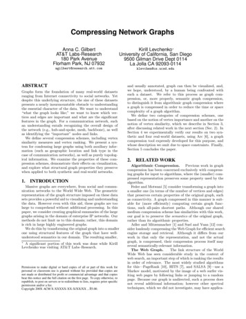
Figure 5: The INET graph before compression (left) and after compression using the Beta weight functionwith the KeepAll algorithm (right). In the compressed graph, important vertices are shown shaded.Figure 6: The AS1239 graph before compression (left) and after compression using Redundant Vertex Elimination followed by the Degree weight function with the KeepOne algorithm. In the compressed graph,merged vertices are shown as diamonds and important vertices are shown shaded.Figure 7: The AS2914 graph before compression (left) and after compression using the Path weight functionwith the KeepOne algorithm. In the compressed graph, important vertices are shown shaded.
Figure 8: The AS3356 graph before compression (left) and after compression using Redundant Vertex Elimination followed by the Beta weight function with the KeepAll algorithm. In the compressed graph, importantvertices are shown shaded.Figure 9: The AS7018 graph before compression (left) and after compression using the Path weight functionwith the KeepAll algorithm. In the compressed graph, important vertices are shown shaded.VERDOS%E%VINET%E%V%AS1239BB %E%V%AS2914BB %E%V%AS3356BB %E%V%AS7018BB %E%Original2937 100 4989 100 3076 100 4859 100 604 100 362 100 2268 100 960 100 453 100 2821 100 624 100 431 100 5298 100 631 100 385 100 2078 100RVE2937 100 4989 100 3074 100 4836 100 553 92 311 86 1605 71 909 95 406 90 2212 78 491 79 303 70 3831 72 576 91 332 86 1337 64Deg/One562551201341 254 247352 232 225301 203 205551 386 349563Beta/One763752321351 366 35 10442 536 419692 264 266491 447 40 10613Path/One351341201371 203 206311 202 204462 203 205561 203 205342Deg/All409 14 574 12 1073 2385 107 18 98 27 390 17 889 85 19 362 13 82 13 79 18 716 14 90 14 82 21 261 13Beta/All522 18 731 15843 1513 134 22 126 35 444 20 136 14 121 27 427 15 96 15 93 22 733 14 102 16 93 24 306 15Path/All280 10 3848 1003 2255 64 11 61 17 1828 657 65 14 2419 70 11 68 16 4498 457 43 11 1085RVE Deg/One552541201351 213 216512 222 204361 203 205 1353 345 328533RVE Beta/All505 17 709 14893 1623 104 17 95 26 315 14 118 12 100 22 329 12 77 12 72 17 643 12 100 16 89 23 259 12RVE Path/One331321201351 203 206462 212 215502 203 174872 213 215352Table 1: A summary of the performance of our compression schemes, showing the number of vertices,backbone vertices, and edges retained by each.
Figure 10: The fraction of backbone vertices in theAS1239 graph under different compression schemes.Figure 12: The fraction of backbone vertices in theAS3356 graph under different compression schemes.Figure 11: The fraction of backbone vertices in theAS2914 graph under different compression schemes.“backbone” label in Rocketfuel dataset, from which the AS1239,AS2914, AS3358, and AS7018 graphs are derived, withthe assumption that backbone routers are intrinsically moreimportant than other types. Figures 10–13 show the fractionof backbone vertices in the original graph and the graph after applying our compression schemes. In all cases, the compression schemes were able to identify the backbone routers,in some cases producing a graph composed exclusively ofbackbone routers. (Note that a decrease in the backbonerouter ratio after applying Redundant Vertex Eliminationindicates that disproportionately more backbone vertices weremerged than ordinary vertices.) In most cases, the Pathweight algorithm (either alone or in conjunction with RVE)produced a graph which consists exclusively of backbonerouters. This suggests that backbone routers are on manyshortest paths between routers, as to be expected! It is interesting to note that the Path weight algorithm employsa measure which tends to compress the graph more than aFigure 13: The fraction of backbone vertices in thedegree-based measure. Not only does this measure removeAS7018 graph under different compression schemes.more extraneous information in the graph but it also retainsmore important information.4.4 Vertex and Edge CompressionBecause we fix the size of K1 at 20 throughout these experiments, it is worthwhile investigating how many verticeseach compression scheme added back (in addition to theimportant ones) to reconnect the graph. This number isthe size of K2 and reflects the connectivity of the impor-
tant vertices. Figure 14 shows for each network and foreach compression scheme the number of additional vertices,expressed as a percentage of the total number of vertices.Because RVE compressed each network poorly, we removedit from the data. INET seems to have a different connectivity structure among its important vertices from the AS andERDOS graphs. Considerably fewer vertices were addedto INET in order to reconnect the important ones. For thereal world networks, the Path algorithm added the fewestvertices which is not surprising as it tends to favor verticesthat lie on a shortest path and, as such, generates importantvertices that are already likely connected.Although each compression scheme operates only on vertices and not on edges, each algorithm does change the number of edges in the graph. Figure 15 shows, for each compression scheme and for each network, the percentage of totaledges retained. This percentage is a reflection of the degreedistribution of the vertices kept in the compressed graphand it shows what percentage of the edges are incident toimportant vertices. We observe that the overall structure ofthis measure is quite similar to the percentage of additionalvertices each scheme requires to reconnect the graph. Notsurprisingly, the more vertices added, the more edges added.What is more interesting is the small relative changes. Forexample, for AS1239, the percentage of additional verticesfor the two schemes Deg (all) and RVE Beta (all) are aboutthe same, 14%. The percentage of edges retained, however,by the two schemes are different, 17% for Deg (all) and 14%for RVE Beta (all). Deg (all) classifies as important verticesthose with a higher degree than RVE Beta (all)’s importantvertices.4.5KeepOne versus KeepAllIn Section 3.1.3 we motivated the KeepAll algorithm byarguing that the KeepOne algorithm does not preserve thedistances between important vertices. Figure 16 shows themost severe distance distortion, which occurred using Pathweight on the ERDOS graph. In practice, the KeepOnedid not differ significantly from the KeepAll algorithm:both generally shifted the distribution but kept its overallshape. As an example, figure 17 shows Path weight on theAS1239 graph.Path (one)Path (all)Original40%30%20%10%05101520Figure 16: The distance distribution on all distinctvertex pairs in the ERDOS graph using Path weightwith the KeepOne algorithm and with the KeepAllalgorithm shown for comparison.Path (one)Path (all)Original40%30%20%10%05101520Figure 17: The distance distribution on all distinctvertex pairs in the AS1239 graph using Path weightwith the KeepOne algorithm and with the KeepAllalgorithm shown for comparison.4.6 Choosing ParametersThroughout the experiments, we fixed the size of K1 tobe 20. One may ask whether this is an optimal choice, orwhether the graph has a “natural” number of importantvertices. Figure 18 shows the fraction of vertices retained asa function of the Beta weight threshold in the range [0.5, 1].Response to the threshold is essentially smooth, with jumpsat small-integer fractions (e.g., 1/2, 2/3, etc.).Figure 19 shows the complementary cumulative distribution of the number of common neighbors between pairs ofvertices. The tail suggests that there are vertices with verylarge sets of common neighbors. Figure 20 shows the complementary cumulative density of a slightly different similarity measure, which is the ratio of the number of common neighbors to the total number of neighbors of a vertex.While this measure is interesting, it does not seem as usefulfor clustering redundant vertices.5.CONCLUSIONThe emergence of large network connectivity datasets 5 0.55 0.6 0.
the data. However even with this aid, these graphs are too large to comprehend without additional processing. In this paper, we consider creating graphical summaries of the large graphs arising in the domain of enterprise IP networks. Our methods do not limit us to this domain; rather, this domain is rich in large highly engineered graphs.