Transcription
SIMPLY-LACED ISOMONODROMY SYSTEMSby PHILIP BOALCHABSTRACTA new class of isomonodromy equations will be introduced and shown to admit Kac–Moody Weyl group symmetries. This puts into a general context some results of Okamoto on the 4th, 5th and 6th Painlevé equations, and showswhere such Kac–Moody Weyl groups and root systems occur “in nature”. A key point is that one may go beyond the classof affine Kac–Moody root systems. As examples, by considering certain hyperbolic Kac–Moody Dynkin diagrams, we findthere is a sequence of higher order Painlevé systems lying over each of the classical Painlevé equations. This leads to aconjecture about the Hilbert scheme of points on some Hitchin systems.CONTENTS1. Introduction . . . . . . . . . . . . . . . . . . . . .2. Modules over the Weyl algebra . . . . . . . . . .3. Symplectic vector spaces . . . . . . . . . . . . . .4. Invariance of spectral invariants . . . . . . . . . .5. Time-dependent Hamiltonians . . . . . . . . . .6. Isomonodromy . . . . . . . . . . . . . . . . . . .7. Nonlinear differential equations . . . . . . . . . .8. Examples . . . . . . . . . . . . . . . . . . . . . .9. Reductions, moduli spaces and relation to graphs10. Additive irregular Deligne–Simpson problems . .11. Example reduced systems . . . . . . . . . . . . .Acknowledgements . . . . . . . . . . . . . . . . . . . .Appendix A: Loop algebras and Adler–Kostant–SymesAppendix B: Harnad duality . . . . . . . . . . . . . .Appendix C: Leading term computation . . . . . . . .Appendix D: Relating orbits . . . . . . . . . . . . . . .Appendix E: Notation summary . . . . . . . . . . . .References . . . . . . . . . . . . . . . . . . . . . . . .110121416232631344851565758596465661. IntroductionThe aim of this article is to introduce and study a new system of isomonodromicdeformation equations. The best known isomonodromy equations are the Schlesingerequations [55] controlling deformations of Fuchsian systems on the Riemann sphere.Geometrically these equations constitute a nonlinear flat connection on a bundleM B Bover a space of parameters (the “times”) B Cm \ diagonals, whereM (O1 · · · Om )//GLn (C)is the symplectic quotient of a product of coadjoint orbits. This nonlinear connectionmay be interpreted as a non-Abelian analogue of the Gauss–Manin connection (cf. [6]Section 7) and admits degenerations into Hitchin-type integrable systems (cf. [23]). ThusDOI 10.1007/s10240-012-0044-8
2PHILIP BOALCHin general one may view an “isomonodromy system” as a system of nonlinear differentialequations obtained by deforming a Hitchin integrable system (and whose solutions willinvolve more complicated functions, such as the Painlevé transcendents, than the Abelianor theta functions involved in solving such integrable systems).The next simplest family of isomonodromy equations are due to Jimbo–Miwa–Môri–Sato (JMMS [27]) and arose as equations for correlation functions of the quantumnonlinear Schrödinger equation. The JMMS equations are the isomonodromic deformation equations for linear differential systems of the form m dRi(1.1) T0 dzz ti1(where T0 is a diagonal matrix) having an irregular singularity at z . A remarkablefeature of the JMMS equations is that there are now two sets of times: one may deformthe pole positions (the ti , as in the Fuchsian case) as well as the eigenvalues of T0 (the“irregular times”). Further Harnad [26] has shown that the JMMS equations admit asymmetry under which one may swap the roles of the two sets of times.In this article we will write down and study the “next simplest” class of isomonodromy equations, which are even more symmetric: in effect the two set of times areextended to k sets of times, all of which may be permuted, and Harnad’s discrete dualityis extended to an action of a continuous SL2 (C) symmetry group. (Further, a Hamiltonian formulation will be given enabling the definition of new τ functions.)One motivation to study such symmetric isomonodromy systems was to better understand and generalise the affine Weyl symmetry groups of the Painlevé equations. Ineffect the Painlevé equations are the simplest examples of isomonodromy equations: theyare the second order nonlinear differential equations which arise as the explicit form ofthe isomonodromy connection when the fibres have dimension two, i.e. dimC M 2.Okamoto has shown that the six Painlevé equations admit certain affine Weyl symmetry groups [45–48], and this is intriguing since the underlying root systems are not immediately apparent from the geometry. For example the simplest nontrivial case of theSchlesinger equations is equivalent to the Painlevé VI equation, which has symmetrygroup the affine Weyl group of type D4 . However no link to the loop group of SO8 ismanifest (one starts with a Fuchsian system with four poles on a rank two bundle). Similarly Painlevé V has affine A3 symmetry group and Painlevé IV has affine A2 symmetryFIG. 1. — Affine Dynkin diagrams for Painlevé equations IV, V and VI
SIMPLY-LACED ISOMONODROMY SYSTEMS3group, as indicated in Figure 1 (the other cases are not simply-laced and will be ignoredhere for simplicity).In the second part of this article (Section 9) we will single out a large class ofgraphs which contains these three graphs, and attach an isomonodromy system to eachsuch graph (and some data on the graph), such that the corresponding Kac–Moody Weylgroup acts by symmetries, relating the corresponding isomonodromy systems. Thus anysuch graph appears as a “Dynkin diagram” for an isomonodromy system. The class ofgraphs for which this result holds contains all the complete k-partite graphs for any k (andin particular all the complete graphs). For example one may ask why there is no secondorder Painlevé equation attached to the pentagon (the affine A4 Dynkin diagram): fromour viewpoint this is because it is not a complete k-partite graph for any k, whereas thetriangle and the square are (as is the four-pointed star).A simple corollary of this way of thinking is that we are able to canonically attachan isomonodromy system of order 2n (i.e. dimC M 2n) to each of the six Painlevéequations for each integer n 1, 2, 3, 4, . . . so that the n 1 case is isomorphic to theoriginal Painlevé system. (These “higher Painlevé systems” look to be completely differentto the well-known “Painlevé hierarchies”).In the remainder of this introduction we will recall more background, summarisethe main result, and describe the JMMS equations from our point of view, serving as themain prototype for the extension we have in mind.1.1. Further remarks and viewpoints. — (1) In 1981 a quite general isomonodromysystem was established by Jimbo–Miwa–Ueno [28], controlling isomonodromic deformations of linear differential systems whose most singular coefficient has distinct eigenvaluesat each pole. This work was revisited from a moduli theoretic viewpoint in [6] and thesymplectic nature of these (JMU) equations was established. More general moduli spaceswere then constructed, without the distinct eigenvalue condition, in [5] (in fact in arbitrary genus and with compatible parabolic structures and stability conditions) and shownto be hyperkähler manifolds. The distinct eigenvalue condition implies that in general theJMU equations are not symmetric, and so here we go back and generalise in a differentdirection the earlier viewpoint of [27]. This is guided by the descriptions in [27, 26, 6]of the moduli spaces involved as symplectic quotients, enabling us to see that some ofthem are isomorphic to (Nakajima) quiver varieties, and thus how the graphs arise fromFIG. 2. — Dynkin diagrams for simply-laced higher Painlevé systems hPIV , hPV , hPVI
4PHILIP BOALCHthe geometry (cf. [16] in the Fuchsian case and [11] Exercise 3 for early examples inthe irregular case). A new viewpoint we have found very useful here is to identify certainquiver varieties (or twisted versions of them) as moduli spaces of presentations of modulesfor the first Weyl algebra.(2) Noumi–Yamada ([41] Problem 5.1) considered the problem of finding systemsof nonlinear differential equations for each affine root system (or more generally for eachgeneralised Cartan matrix) on which the corresponding Weyl group acts as Backlundtransformations. As an example in [42] (see also Noumi’s ICM talk [40]) they wrotedown a sequence of isomonodromy equations for each of the type A affine Weyl groups,generalising the Painlevé IV and V equations. See also various articles of Y. Sasano suchas [54]. (Note they have also found [43] a direct link between PVI and SO(8).) Their workis in a sense orthogonal to ours: although we consider a much larger class of Kac–Moodyroot systems, whereas they only construct systems in certain affine Kac–Moody cases,the intersection of the set of our graphs with theirs is amongst the usual second orderPainlevé equations. (I do not know if there is some common generalisation.)(3) The graphs we are using give a reasonably efficient way to start to classifysome isomonodromy systems (or at least to tell when they might be isomorphic). Somefour dimensional examples were found in this way in [10] by looking amongst the hyperbolic Kac–Moody graphs (the next simplest class after the affine ones). Not everyisomonodromy system will be simply-laced though of course. Some other possible approaches to such questions are as follows. (i) Recall that Cosgrove (e.g. in [14]) has donemuch work classifying higher order equations with the Painlevé property although his approach seems difficult for higher rank equations (e.g. sixth order). (ii) On the other handMalgrange [35] and Umemura [57] have introduced a nonlinear differential Galois theory which one might hope would help with such classification, although it turns out thatthe strength of their theory is its vast generality and present results suggest it does noteven distinguish amongst the six Painlevé equations themselves (when they have genericparameters).1(4) In essence we are associating what might be called a “wild non-Abelian Hodgestructure” to a certain class of graphs with some extra data on them. This structure consists of a hyperkähler manifold M (as in [5]) which in one complex structure is a modulispace of meromorphic connections and in another is a space of meromorphic Higgsbundles. The isomonodromy system is naturally associated to this structure (it controlsthe isomonodromic deformations of the meromorphic connections). It seems that thework of S. Szabo [56] (interpreting certain Fourier–Laplace transforms as Nahm transforms) can be extended to show that the full hyperkähler metric is also preserved by allthe Kac–Moody Weyl group symmetries.1One could see this attempt to classify such nonlinear algebraic differential equations as a basic step in “differentialalgebraic geometry”—the extension of algebraic geometry obtained by allowing derivatives in the equations—the isomonodromy equations should form a basic class of objects to be studied, much as Abelian varieties or Calabi–Yau manifoldsare in classical algebraic geometry. On the other hand one can view this subject as a half-way step to “noncommutativealgebraic geometry”.
SIMPLY-LACED ISOMONODROMY SYSTEMS5FIG. 3. — Complete k-partite graphs from partitions of N 6 (omitting the stars G (1, n) and the totally disconnectedgraphs G (n))1.2. Summary of main result. — The main result involves a class of graphs that wewill call supernova graphs (cf. Definition 9.1), generalising the class of star-shaped graphs. is a supernova graph with nodes In brief GI if for some k there is a complete k-partite subgraph G G with nodes I I, and G is obtained from G by gluing on some legs. Inturn recall a complete k-partite graph is a graph whose nodes IjI j Jare partitioned into parts parameterised by a set J with J k, and two nodes of G arejoined by a single edge if and only if they are not in the same part. be a supernova graph and choose data d,λλ, a, consisting of:Let G(1) An integer di 0 for each node i I, (2) A scalar λi C for each i I, such that λi di 0,(3) A distinct point aj of the Riemann sphere for each part j J.Theorem 1.1. — There is an isomonodromy system(1.2)λ, d, a) B BM st (λ
6PHILIP BOALCH where the space of times is B j J (C Ij \ diagonals). It controls isomonodromic deformations ofcertain linear differential systems on bundles of rank di ,(1.3)i I\I where I I is the part with aj . and λi 0 then there is an isomorphism of isomonodromy systems If i I is a node of Gλ, d, a) B λ), si (d), a BM st (λ M st ri (λwhere si , ri are the simple reflections (and dual simple reflections) generating the Weyl group of the Kac– .Moody root system attached to the graph G If g SL2 (C) then there is an isomorphismλ, d, a) BM st λ, d, g(a) B M st (λof isomonodromy systems, where g acts on a by diagonal Möbius transformations.Also, in Section 10, precise criteria involving the Kac–Moody root system will beestablished for when the spaces M st are nonempty—this is an additive, irregular analogue of the Deligne–Simpson problem. Notice in particular that the action of SL2 (C)enables us to change the ranks appearing in (1.3), by moving different points aj to .Once we have this possibility it is straightforward to obtain all the reflections geometrically. (This extends the viewpoint of [8, 9] which derived the action of the Okamotosymmetries of Painlevé VI on linear monodromy data from Harnad duality/Fourier–Laplace.)1.3. Prototype: The lifted JMMS equations. — By writing the (lifted) JMMS equationsin a slightly novel way we will show how graphs appear naturally. In particular we willexplain how the square (which Okamoto attached to Painlevé V) emerges from the viewpoint of [27] Appendix 5. Our main result is obtained by extending this to include thetriangle.Choose two finite dimensional complex vector spaces W0 , W and consider thespace M Hom(W0 , W ) Hom(W , W0 ). The (lifted) JMMS equations govern how(P, Q) M should vary with respect to some times T0 , T , and we will write theseequations in the following form:(1.4)dQ QPQ QPQ T0 QdT dT0 QT dP PQP PQP T PdT0 dT PT0 .Here T0 , T are semisimple matrices T0 End(W0 ), T End(W ) which mayhave repeated eigenvalues, but are restricted so that no further eigenvalues are allowed
SIMPLY-LACED ISOMONODROMY SYSTEMS7to coalesce, and the corresponding eigenspace decompositions of W0 , W are held constant. The tilde operation appearing in (1.4) is defined as follows: if R End(Wi ) thenR : ad 1Ti [dTi , R]which is a one-form with values in the image in End(Wi ) of adTi . (To see this makes sensenote that adTi is invertible when restricted to its image.) These equations are known tohave the Painlevé property and special cases include the fifth and sixth Painlevé equations.Indeed for example in a special case they imply the Schlesinger equations: if one restrictsto the case when T0 0 then (1.4) simplifies todQ QPQ,dP PQP. It follows immediately that if we write T ti Idi where Idi is the idempotentfor the ith eigenspace of T and set Ri QIdi P End(W0 ) thendRi [Ri , Rj ]d log(ti tj )j iwhich are the Schlesinger equations. They govern the isomonodromic deformations ofa logarithmic connection on the vector bundle W0 P1 P1 . In general the JMMSequations govern the isomonodromic deformations of a meromorphic connection (corresponding to the differential system (1.1)) on the vector bundle W0 P1 P1 having anirregular singularity of Poincaré rank one and arbitrarily many logarithmic singularities.Although quite general nonlinear isomonodromy equations have been written down byJimbo–Miwa–Ueno [28], the JMMS equations are notable since they have the followingsymmetry (now quite transparent in the way we are writing the equations):Theorem 1.2 (Harnad duality [26]). — The permutation(W0 , W , P, Q, T0 , T ) (W , W0 , Q, P, T , T0 )preserves the JMMS equations.This is remarkable since it implies that the same equations also control isomonodromic deformations of a connection on the vector bundle W P1 P1 , which ofcourse will in general have different rank.Our basic aim is to show that the JMMS equations have a natural generalisationthat admits an enriched symmetry group. To describe the picture let us first describe thecombinatorics of Harnad’s duality in terms of graphs. First consider the graph with twonodes labelled by 0 and connected by a single edge. We put the vector space Wj at the
8PHILIP BOALCHnode j for j 0, and view the maps P, Q as maps in both directions along the edge.At this level (up to a sign) Harnad duality simply flips over the graph.The next step (which enables us to see the link to Dynkin graphs) is to refine theabove graph by splaying each node according to the eigenspaces of the times T0 , T . Inother words suppose Wj i Ij Vi is the eigenspace decomposition of Tj for j 0, .Then we break up the node corresponding to W0 into I0 nodes and thereby splay thegraph (and similarly at the other node), as in the diagram below (for the case I0 3, I 2):Note that the class of refined graphs which arise in this way are precisely the completebipartite graphs. Now the fifth Painlevé equation is equivalent to a basic case of the JMMSequations (appearing in the title of [27]): it occurs when both W0 and W have dimensiontwo and each time Tj has two distinct eigenvalues. The crucial observation then is that inthis case the refined graph is a square, i.e. the affine Dynkin diagram A(1)3 that Okamotoassociated to Painlevé V appears almost directly from the work of JMMS.This is more than a coincidence since, as we will confirm, Harnad’s duality (andthe well-known Schlesinger/Backlund transformations) yield the Okamoto symmetries.Moreover we see how to put this in a more general context since any complete bipartitegraph also appears in the same way.The final step “reduction” (see Section 9) is to choose an adjoint orbit Ŏi End(Vi ) for each node of the refined graph and quotient by the symmetry groupFIG. 4. — How A(1)3 appears in the graphical approach to the JMMS system
SIMPLY-LACED ISOMONODROMY SYSTEMS9 GL(Vi ). In terms of graphs this will correspond to gluing a leg (a type A Dynkingraph) onto each node of the refined graph: the resulting graph is the Dynkin diagram ofthe Kac–Moody root system whose Weyl group naturally acts on the nonlinear equations.1.4. Generalisation. — The generalisation we have in mind involves replacing theinitial graph in the JMMS story above (the interval) by an arbitrary complete graph. (Recallthat the complete graph with k nodes has exactly one edge between any two vertices.)Each node of the graph will be labelled by a distinct element aj C { } of theRiemann sphere. Thus if J is the set of nodes we may view J as a subset of the Riemannsphere. (We will see below that plays a distinguished role.) In the case of the JMMSequations above we had J {0, }. As above we attach a vector space Wj to each nodej J and consider a set of times which are semisimple elements Tj End(Wj ) for eachj J. The set of unknown variables in the nonlinear equations, generalising (P, Q) above,again consists of the linear maps in both directions along each edge:Bij Hom(Wj , Wi ),for all i j J.The integrable nonlinear equations we will find governing these then have the form:dBij X ik Bki Bij Bij Bjk Xkj dTi Xik Bkj Bik Xkj dTj Xik dTk Xkj /φijk Jplus some terms linear in Bij that we will neglect in the introduction, where φij is a complex number depending only on the embedding J C { } and Xij φij Bij . (Observethat the three quadratic terms are absent in the original JMMS equations.)The remainder of the story is then similar to above: we splay the nodes of thecomplete graph according to the eigenspaces of the times Tj to obtain a refined graph.(The class of graphs which arise in this way is exactly the class of complete k-partitegraphs.) Then we reduce as above, gluing on some legs, to obtain a graph whose Kac–Moody Weyl group acts. The simplest case, with k 3 and each Wj of dimension one,is equivalent to the fourth Painlevé equation (and the refined graph, which in this caseequals the unrefined graph, is the triangle, agreeing with Okamoto).FIG. 5. — The sequence of complete graphs
10PHILIP BOALCH2. Modules over the Weyl algebraThis section describes the class of modules over the first Weyl algebra that we wishto consider. By taking this viewpoint, rather than just that of meromorphic connections,more symmetries are apparent. (Appendix B explains how this generalises Harnad’s duality.) Choose three n n complex matrices α, β, γ and consider the matrixM α βz γwith values in the first Weyl algebra A1 C z, , where d/dz.We wish to study (local) systems of differential equations of the formM(v̂) 0for a vector v̂ of holomorphic functions. This may be rephrased as the local system ofholomorphic solutions of the (left) A1 -module N defined by the exact sequence(·M)An1 An1 N 0.We will restrict to the case where α and β are commuting diagonalisable matriceswhose kernels intersect only at zero. This class of modules is clearly preserved under theFourier–Laplace transform, and in fact by more general symplectic transformations(2.1)( , z) (a bz, c dz)where ad bc 1:Lemma 2.1. — If α and β are two commuting semisimple matrices whose kernels intersect onlyat zero, then so areaα cβand bα dβfor any complex numbers a, b, c, d with ad bc 1.Proof. — In each joint eigenspace the corresponding pair of eigenvalues (αi , βi ) isa nonzero point of C2 . We are acting on this element of C2 by an invertible matrix so itwill remain nonzero. Thus such a module determines a finite number of points ai : [ βi : αi ] P : P (C) of the projective line (the minus sign appearing here will be useful later). We labelthis sphere P (and call it the “Fourier sphere”) to avoid confusion later with the Riemannsphere P1z on which z is a local coordinate. Let J be the set of such points of P, and letk J be the number of points so obtained (which is in general less than the number ofjoint eigenspaces, since two pairs of eigenvalues may differ by an overall scalar). For each1
SIMPLY-LACED ISOMONODROMY SYSTEMS11point j J there is an associated subspace Wj V : Cn (the joint eigenspaces havingpairs of eigenvalues lying over j), so that V j J Wj .We will further assume for each j that the component of γ in End(Wj ) is semisimple.Let [1 : 0] be the point of P where αi 0, corresponding to the kernel of α(we are not assuming J; this kernel may be trivial). Any other point of P correspondsto a complex number (ai βi /αi C); we identify P with C { } in this way.By multiplying M on the left by a constant invertible matrix, we may then normalise M uniquely so it is of the form 01 0(2.2)M z γ End(W U ) A110 A where Uj V Wj i J\{j} Wi . Here A j aj Idj End(U ) where Idj is theidempotent for Wj V. The decomposition of V allows us to decompose End(V) as End(V) Hom(Wi , Wj ) End(Wj )i j Jj Jand so we may decomposeγ γ δ(γ )with respect to this decomposition. We will also write (after normalisation) 0 PC End(W U ).(2.3)δ(γ ) T ,γ Q BTThus α, β, γ determine linear maps B, T End(U ), C End(W ) and P : U W and Q : W U and by assumption C and T are semisimple.The corresponding system of differential equations then takes the form(2.4) v Az B T Q(z C) 1 P vfor a holomorphic function v (with values in U ). This system corresponds to the meromorphic connection on the trivial holomorphic bundle on P1 with fibre U determinedby the matrix of meromorphic one-forms:(2.5)A Az B T Q(z C) 1 P dz.In general this connection will have a pole of order three (irregular singularity of Poincarérank two) at z and a simple pole (Fuchsian singularity) at each eigenvalue of C.If instead we first perform a symplectic transform (2.1) before passing to the connection (2.5) then a different connection will be obtained, usually on a different rankbundle. Indeed if the transform moves j J to then the resulting bundle will have fibre
12PHILIP BOALCHUj V Wj . On the other hand (after a generic symplectic transform) it will have fibreV—if no points of J are at . Thus in general connections will be obtained on k 1 bundles of different ranks (and in fact on each of these bundles a whole family of connectionsis obtained corresponding to the affine subgroup of SL2 (C) stabilising P).Our basic aim is to show that the isomonodromic deformations of such connections (on different rank bundles) are governed by the same system of nonlinear differentialequations when we vary T and C.3. Symplectic vector spacesSuppose (as above) we have a finite dimensional complex vector space V graded bya finite set J, so that V j J Wj for subspaces Wj . Consider the complex vector space M : End(V) Hom(Wi , Wj )i j Jof linear maps in both directions between each pair of distinct vector spaces Wj .Now suppose we have an injective map a : J P C { } (as above) so we mayidentify J with its image in P. Thus in effect we have a vector space Wp for each p P/ J). We write ai a(i) for the complex number corresponding to(taking Wp {0} if p i J \ { }. Then we may define a complex symplectic structure on M by the formulaω ωa Tr(dBij dBji )Tr(dBi dB i ) 2(a a)iji j J\{ }i J\{ }where Bij Hom(Wj , Wi ). We will sometimes write M Ma when we think of it as acomplex symplectic manifold with the symplectic form ωa . If we define constants φij Cfor i, j J so that φii 0, φij (ai aj ) 1 if i, j and φi 1 φ i thenω 1 1 φij Tr(dBij dBji ) Tr(dXij dBji )2 i,j J2 i,j Jwhere we have defined Xij φij Bij Hom(Wj , Wi ) for all i, j J.Now suppose we have matrices α, β, γ as above, and we normalise them as in (2.2).Then for i j J we will identify Bij above with the component of γ in Hom(Wj , Wi ), sothat P has components B i , Q has components Bi and the Hom(Wj , Wi ) componentof B is Bij (for i j J \ { }). In these terms(3.1)1ω Tr(dQ dP) Tr(dX dB)2where X ad 1A (B) Im(adA ) End(U ).
SIMPLY-LACED ISOMONODROMY SYSTEMS13Finally if we define φ( ) where φ : End(V) End(V) is the linear map givenin components by (Bij ) (φij Bij ) (so that Xij is always the Hom(Wj , Wi ) component of) or in other words 0 P0 P , End(W U ),Q XQ Bthen the symplectic form is(3.2)1ω Tr(d2 d ).Note the basic property of φ, that it is skew-adjoint: Tr(φ(E)F) Tr(Eφ(F)).In particular this implies Tr( ) 0. The key fact about these symplectic forms is thefollowing:Proposition 3.1. — The symplectic form ω on M is equivariant under the symplectic transformations (2.1) of M.Said differently, given an injective map a : J P and a symplectic matrix g SL2 (C) weobtain a map ϕ : Ma Mg·a (by acting on M with g and renormalising). We are claimingthat ϕ is symplectic.Proof. — The group SL2 (C) is generated by (i) the scalings ( , z) ( /c, cz) forc C , (ii) the shearings ( , z) ( cz, z) for c C, and (iii) the Fourier–Laplacetransform ( , z) ( z, ) (beware this convention is sometimes taken to be the inverseFourier–Laplace transform). Note that (i) and (ii) correspond (on the level of connections(2.5)) respectively to scaling the coordinate z and to tensoring by the connection czdz onthe trivial line bundle.For (i), the resulting action on is 0 P0 P/c Q BcQ cBand aj c2 aj for all j. Thus becomes ε where ε diag(1/c, c) and in turn it followsthat becomes ε 1 . Thus from (3.2), this transformation leaves ω unchanged.For (ii), γ is unchanged and each aj is replaced by aj c, which again fixes ω.For (iii) recall W0 is the kernel of A (or equivalently of β), so we may write 10 P0 Pr ,(3.3)β 0 Q 0 0 B0r End W W0 VrQ r Br0 Brr Ar
14PHILIP BOALCHwhere Vr then find β,(3.4)j 0, Wjis the “rest of V”. After Fourier–Laplace and renormalising webecome: 0 1β , A 1r εwhere ε diag(1, 1, A 1r ). Noting that the roles of W0 and W have been swapped(and ai 1/ai ), we find directly thatLemma 3.2. — Under the Fourier–Laplace transformThus ω in (3.2) is clearly preserved.becomes ε 1 . In other words the above formulae define a symplectic action of SL2 (C) on thesymplectic vector bundle M P J \ (diagonals) (with fibres Ma ) covering the standardaction (diagonal Möbius transformations) on the base P J \ (diagonals).4. Invariance of spectral invariantsAs is by now well known, isomonodromy systems have degenerations (dating backat least to [23]) which are isospectral integrable systems (solvable by spectral curve methods i.e. in terms of Abelian functions). Here we will briefly touch on this in our context,focusing on the results we will need elsewhere in this article (our main interest being theisomonodromic system, requiring in general more complicated functions to solve them).This extends some work of Adams–Harnad–Hurtubise [1].Suppose we fix T and A as above (except in this section we do not need to assume T, A) denote the ring of functions on M generated by theT is semisimple). Let I I ( coefficients of the polynomialP (λ, z) det(z C) de
SIMPLY-LACED ISOMONODROMY SYSTEMS 5 FIG.3.—Completek-partite graphs from partitions of N 6 (omitting the stars G (1,n) and the totally disconnected graphsG (n)) 1.2. Summary of main result. — The main result involves a class of graphs that we will call supernova graphs (cf. Definition 9.1), generalising the class of star-shaped graphs. In brief G is a supernova graph with .