Transcription
Drawing Power Law Graphs using a Local/Global Decomposition Reid AndersenFan ChungUniversity of California, San DiegoUniversity of California, San DiegoLinyuan LuUniversity of South CarolinaAbstractIt has been noted that many realistic graphs have a power law degree distribution and exhibit the smallworld phenomenon. We present drawing methods influenced by recent developments in the modeling ofsuch graphs. Our main approach is to partition the edge set of a graph into “local” edges and “global”edges, and to use a force-directed method that emphasizes the local edges. We show that our drawingmethod works well for graphs that contain underlying geometric graphs augmented with random edges,and demonstrate the method on a few examples. We define edges to be local or global depending onthe size of the maximum short flow between the edge’s endpoints. Here, a short flow, or alternativelyan -short flow, is one composed of paths whose length is at most some constant . We present fastapproximation algorithms for the maximum short flow problem, and for testing whether a short flow of acertain size exists between given vertices. Using these algorithms, we give a fast approximation algorithmfor determining local subgraphs of a given graph. The drawing algorithm we present can be applied togeneral graphs, but is particularly well-suited for numerous small-world networks with power law degreedistribution.1IntroductionAlthough graph theory has a history of more than 250 years, it was only recently observed that many realisticgraphs from disparate areas satisfy the so-called “power law”, where the fraction of nodes with degree k isproportional to k β for some positive exponent β. Graphs with power law degree distribution are prevalentin the Internet, in communication networks, social networks and in biological networks [1, 2, 4, 5, 6, 9, 10,13, 15, 20, 23, 24, 27]. Many real examples of networks also exhibit a so-called “small world phenomenon”consisting of two distinct properties — small average distance between nodes, and a clustering effect wheretwo nodes sharing a common neighbor are more likely to be adjacent. It was shown in [11] that a randompower law graph has small average distance and small diameter. However, random power law graphs do notadequately capture the clustering effect.In [3], the authors introduced a hybrid graph model where a random power law graph called the globalgraph is added to an underlying local graph. A local graph is a graph where the endpoints of each edge arehighly locally connected by large short flows. In particular, a graph is said to be (f, )-local if the endpointsof each edge are connected by an -short flow of size f . Random geometric graphs and d-dimensional gridgraphs are good examples of local graphs for various parameters. Given an arbitrary graph G, we can chooseparameters f and and define the local graph of G to be its largest (f, )-local subgraph, providing a wayto partition G into local and global edges. The main result of [3] is that the local graph of a hybrid graph is Research1Asupported in part by NSF Grants DMS 0100472 and ITR 0205061conference version appeared in Proceedings of the Twelfth Annual Symposium on Graph Drawing, 20041
equal to the original local graph up to a small error, indicating that local graphs are robust to the additionof random edges.In this paper we demonstrate that partitioning a graph into local and global edges based on local connectivity can be done quickly, and can be useful in graph drawing. To obtain local/global partitions for largegraphs, we present an approximation algorithm for computing the local graph. We also give a new algorithmfor the fundamental problem of computing the maximum short flow between given vertices. The numberof iterations required in our maximum short flow algorithm depends on the value fopt of the maximumshort flow. We also give a new algorithm for the problem of local connectivity testing, where we wish todetermine whether there exists a short flow of a certain size ftest between given vertices. The number ofiterations required by our testing algorithm is determined by ftest and not fopt , so testing local connectivitycan be done significantly faster than computing the maximum short flow. Our algorithms are based on themaximum multicommodity flow algorithm of Garg and Könemann [17].After obtaining a local/global partition, we use it by modifying a standard force-directed algorithmto emphasize local edges. We demonstrate that this method produces improved drawings for graphs thatcontain underlying geometric graphs augmented with random edges. This is theoretically supported, sincethe robustness of the local graph implies that most of the edges in the underlying geometric graph will beclassified as local, while most of the edges from the random graph will be classified as global.We also present a drawing method based on a more sophisticated partition that reflects other aspectsof the structure of power law graphs. For example, it was shown in [11] that a random power law graphhas roughly an “octopus” shape, with a dense “core” and a myriad of “tentacles” attached. While the coreitself may be a dense graph that is not amenable to most drawing methods, our algorithm takes advantageof the local subgraph and the sparse tree-like structures in the tentacles, yielding improved drawings. Thispartition extends the class of graphs for which the local/global partition is useful to many realistic networkswhere some notion of closeness between vertices is reflected in the edge set.2PreliminariesIn [3], the authors introduced local graphs, which are graphs where the endpoints of each edge are highlylocally connected by a large short flow. In this section we introduce short flows and define local graphs. Wewill also state a theorem showing that local graphs are robust to the addition of random edges. Throughoutthe paper, the graphs we consider are undirected and unweighted.2.1Short Flows and Local ConnectivityThere are a number of ways to define local connectivity between two given vertices u and v. A naturalapproach is to consider the connectivity through paths whose length is at most some fixed constant , whichwe will call -short paths or simply short paths. The path connectivity a (u, v) is the maximum size ofan -short collection of edge-disjoint u v paths. The cut connectivity c (u, v) is the minimum size of an -short u v cut, a set of edges whose removal leaves no -short u v paths. The analogous version ofMenger’s theorem does not hold when we restrict to short paths— a (u, v) and c (u, v) are not necessarilyequal. However, it is easy to see that the trivial relations a c · a still hold.Both a (u, v) and c (u, v) are difficult to compute. In particular, computing the maximum number ofshort disjoint paths is N P-hard if 4 [19]. In light of this result we will define local connectivity based onmaximum short flow, which we will define shortly, and which can be efficiently computed, as we will showin Section 3.2
An -short flow is a linear combination of -short paths where each edge has congestion at most 1. Ifwe let A be the incidence matrix where each column represents a -short path from u to v and each rowrepresents an edge in the graph, then finding f (u, v), the maximum -short flow between u and v, can beviewed as the following linear program.f (u, v) max{ 1T x Ax 1, x 0 }.(1)The linear programming dual of the maximum short flowP problem is a fractional cut problem. An -shortfractional cut is a weight function w : E R such that e P c(e) 1 for every -short u Pv path P . Thedual of the -short maximum flow problem is to find an -short fractional cut that minimizes e G c(e). Welet w (u, v) denote the size of a minimum -short fractional cut, and note that LP duality impliesa (u, v) f (u, v) w (u, v) c (u, v).(2)Definition 1 Two vertices u and v are (f, )-connected if f (u, v) f .Since all the coefficients in the incidence matrix, cost vector, and constraint vector in the problemformulation (1) are nonnegative, the maximum short flow problem belongs to a special subset of linearprograms called fractional packing problems, for which there exist general techniques that often lead topolynomial time algorithms [29]. In Section 3 we present a fast primal-dual algorithm for computing themaximum -short flow. We will also present an algorithm to test whether two vertices are (f, )-connected,which can be significantly faster than computing the maximum -short flow.2.2Mengerian Theorems for Short PathsIt was mentioned previously that a (u, v) and c (u, v) are not necessarily equal. It is an open problem todetermine how much these quantities can differ with respect to . It was shown by Lovász, Neumann-Lara,and Plummer [26] that c 2 · a . Boyles and Exoo [8] have given a family of graphs where c 4 · a . Theirresults were stated for the case of vertex-disjoint paths, but the results convert easily to the edge-disjointcase which we are considering. We now present a simple construction showing that c 3 · a for infinitely many , improving the best known lower bound. We conjecture that c 3 o(1) · a for all graphs.Theorem 1 For every there exists a graph such that a (u, v) 1 and c (u, v) 3 .Proof: Consider a path P x1 . . . x2n of length 2n 1. We add 2n disjoint paths of length 2 between eachpair of adjacent vertices xi and xi 1 . Call this graph G2n , and let u x1 and v xn .We refer to the edges of P as base edges. It is easy to see that an s t path using at most k base edgeshas length at least (4n 2) k. If we set 3n 2, then every -short path must use at least n base edgesso that its length is at most (4n 2) n 3n 2 . Since there are only 2n 1 base edges, any two -short paths must intersect in a base edge, so a (u, v) 1. We now consider the size of a minimum -shortcut C. Without loss of generality we can assume that C cuts only base edges. If C cuts n 1 or fewer baseedges, then n base edges remain and the path that proceeds from xi to xi 1 by taking a base edge wheneverpossible has length at most (4n 2) (n) 3n 2 . Thus, c (u, v) n, and soc (u, v) n · .3n 23It is not hard to modify the above construction to obtain examples for 3n 1 and 3n withc (u, v) 3 . We can increase by 1 or 2 without changing a (u, v) or c (u, v) if we add a vertex x0 , letu x0 , and connect x0 to x1 with 2n paths of length 1, or 2n paths of length 2.3
2.3Local GraphsDefinition 2 A graph L is (f, )-local if for each edge (u, v) in L, the endpoints u and v are (f, )-connectedin L.For example, the toroidal grid graph Cn Cn is (3, 3)-local. This graph is also (4, 5)-local, which is slightlyless obvious and highlights the difference between a (u, v) and f (u, v). A 4-short flow of size 5 between theendpoints of a grid edge is shown in the figure below. The correct combination to take is 1 of the path inthe grid on the left, and (1/2) of each path in the remaining grids.vvuuvuvuFigure 1: A 5-bounded flow of size 4 between endpoints of a grid edge.The union of two (f, )-local graphs is (f, )-local, and so there is a unique largest (f, )-local subgraph ofG, which we denote Lf, (G). In Section 4 we will present approximation algorithms for computing Lf, (G).It is important to note that Lf, (G) is not necessarily connected.2.4Random Graphs with Specified Expected Degree SequenceA random graph G(w) with specified expected degree sequence w (w1 , wP2 , . . . , wn ), is formed by includingeach edge vi vj independently with probability pij wi wj ρ, whereρ (wi ) 1 . It is easy to check thatP2vertex vi has expected degree wi . We assume that maxi wi k wk so that pij 1 for all i and j. Thiscondition also implies that the sequence wi is graphical [14] if the wi are integers. This model has a non-zeroprobability of self-loops, but the expected number of loops is of lower order than the total number of edges.The typical random graph G(n, p) on n vertices with edge probability p is a random graph with expecteddegree sequence w (pn, pn, . . . , pn). For a subset S of vertices, we defineXXVol(S) wiandVolk (S) wik .vi Svi SLet d denote the average degree V ol(G)/n, and let d denote the second-order average degree Vol2 (G)/Vol(G).We also let m denote the maximum weight among the wi .2.5Robustness of Local GraphsWe consider how the local graph Lf, (G) changes with the addition of random edges. In particular weconsider the addition of the edge set of a random graph G(w) with a specified expected degree sequence.The following theorem states that local graphs are robust to the addition of these edge sets, provided therandom graph is not too dense. Graphs formed by the union of a local graph L and a random graph G(w)were considered in [3], and were there called hybrid graphs.4
Theorem 2 Let L be an (f, )-local graph with maximum degree M . Let G(w) be a random graph from the and maximum weightspecified expected degree model with averageweight d, second order average weight d,Sm. Let H be the hybrid graph H G L, and let Lf, (H) be the unique largest (f, )-local subgraph of H.If d satisfiesd nα ndm2 1/ n 3/f for some constant α 0,Then with probability 1 O(n 1 ): edges.1. L0 \ L contains O(d)2. dL0 (x, y) 1 dL (x, y) for every pair x, y L.The proof of this theorem is contained in [3].3Fast Algorithms for Short Flow ProblemsGarg and Könemann [17] gave simple combinatorial algorithms for maximum multicommodity flow, maximum concurrent flow, and general fractional packing problems. We present a simple primal-dual approximation algorithm for the maximum short flow problem based on their techniques. The number of iterationsrequired by our algorithm is smaller than the number required by the algorithms for maximum multicommodity flow or general fractional packing problems. This is because the number of iterations in our algorithm canbe bounded in terms of f (u, v), whereas the stated bounds for the multicommodity flow algorithm dependson M .Since we are computing -short flows, our algorithms only need to consider the edges involved in some -short u, v path, which are all contained in the subgraph N /2 (u) N /2 (v). Thus, our running times willbe bounded in terms of m, the number of edges in the small subgraph N /2 (u) N /2 (v), and not on M , thenumber of edges in the entire graph.In our applications, we will be repeatedly testing whether two given vertices are (f, )-connected for someconstants f and , which we call the local connectivity testing problem. We combine our maximum shortflow algorithm with a greedy path selection algorithm to obtain an algorithm for local connectivity testingwhere the number of iterations required depends on the constant f rather than f (u, v). Thus, in many caseswe can test local connectivity much faster than we can compute the maximum short flow.3.1Computing the Maximum Short FlowMaximum Short Flow:The algorithm produces an -short flow f by routing one unit of flow at each time step.Initially,Let w0 be a weight function w0 : E R assigning weight δ to every edge in N /2 (u) N /2 (v).Let f0 be the empty flow.At each time step i,Let p(i) be an -short path of minimum weight with respect to the current weight function wi .Let α(i) be the weight of this path.Modify f by routing 1 unit of flow on p(i),5
Modify the weight function by setting wi 1 (e) wi (e) · (1 ) for each edge e p(i).The procedure stops at the first time step t when α(t) 1.The flow f (t) is then scaled by the maximum edge congestion to obtain a feasible -short flow fˆ.Finding a minimum-weight -short path can be done easily:For each k 0 . . . and each vertex x,Let w(x, k) be the minimum weight of a path from u to x of length less than or equal to k.Let p(x, k) be its predecessor on one path achieving this minimum.Compute the values of w( , k 1) and p( , k 1) from the values of w( , k).Once all the w(x, k) and p(x, k) are computed, we can obtain the minimum weight path,backward from v to u, by letting x0 p(v, ) and xi p(xi 1 , i) until we reach u.Thus we obtain a minimum-weight -short path in time Tmwp O(m ). 2Theorem 3 The algorithm Maximum Short Flow produces a feasible flow fˆ (u, v) which is a (1 ) 1approximation to the maximum short flow f (u, v). The algorithm runs in time f (u, v) 2 log Tmwp ,where Tmwp O(m ) is the time required to find a minimum-weight -short path in a weighting of thesubgraph Gu,v, , and m is the number of edges in N /2 (u) N /2 (v).The analysis of the approximation guarantee for the maximum short flow algorithm is nearly identical tothe analysis for the maximum multicommodity flow algorithm in Garg and Könemann [17], but the analysisof the number of iterations required contains a significant difference. For completeness, we include the fullanalysis here.Proof of the Papproximation guarantee:PLet D(w) e w(e) be the total amount of weight in the weight function w and let α(w) minp e p w(e)be the minimum weight of any -short path with the weight function w. Let D(i) D(wi ) and α(i) α(wi ).At each step i 1,D(i) Xwi (e)e Xwi 1 eXw(e)e p(i) D(i 1) · α(i 1),and thusD(i) D(0) iXα(k 1).(3)k 1Consider β minw D(w)/α(w), where the minimum is taken over all possible weight functions whereα(w) 6 0. Since we can scale any such weight function by α(w) 1 to obtain an -short fractional cut, β is theoptimum value of an -short fractional cut. Now consider the weight function wi w0 where the initial weightsδ are subtracted from each edge that has been used to route flow in fi . We have D(wi w0 ) D(i) D(0)and α(wi w0 ) α(i) δ . Thus,β D(wi w0 )D(wi w0 ) ,α(wi w0 )α(i) δ 6
and so D(i) D(0) β(α(i) δ ). We substitute this in equation (3) to obtainα(i) δ i Xα(k 1),βk 1and since α(i) is as large as possible when α(i 1) is as large as possible, α(i) α(i 1)(1 ) α(i 1)e /β .βSince α(0) δ we obtainα(i) δ e i/β .Also, α(t) 1 by the stopping condition, so1 α(t) δ e t/β .By taking logs we obtain β 1 .tln( δ )(4)Every edge e has wt (e) 1 , since the last time e was increased it was on a path of length strictly lessthan 1, and its weight was increased by a factor of 1 . Since w0 (e) δ, it follows that the weight of e can1 be increased at most log1 1 δ times, and thus the total flow through e is at most log1 δ . Scaling thetflow ft by the maximum congestion yields a feasible flow fˆ of value at least log 1 .1 δTherefore the approximation ratio γ isββ1 log1 .ˆtδfSubstitute the bound on β/t from equation (4) to obtainln 1 1 δlog 1 11 .δln(1 ) ln( δ ))ln( δ 1/ if we set δ (1 ) (1 ) . With this δ we haveγ The ratioln 1 δ1ln( δ )is (1 ) 1γ (1 ) 2 .(1 ) ln(1 )(1 )( 2 /2)Analysis of the running time: Each edge can have its weight multiplied by (1 ) at most log1 1 δ timesuntil it’s weight reaches 1 and it can not be further increased. If C(u, v) is an -short cut, then at everytime step some edge in C(u, v) has its weight multiplied by (1 ). Thus, the algorithm performs at mostc (u, v) log1 1 δ iterations before terminating. To obtain the stated approximation ratio, the initial weightδ is set to (1 )((1 ) ) 1/ . Thus the number of iterations required is at mostc (u, v) log1 1 12 c (u, v) log1 (1 ) c (u, v) 2 log2 .δ (5)The number of iterations can also be bounded in terms of the flow by applying the bound c (u, v) 2 ·f (u, v),which was mentioned in Section 2.1. The number of iterations required is then f (u, v) 12 log2 . The resultfollows.It should be noted that our bound on the number of iterations depends crucially on the fact that alledge capacities are equal to 1. It is not hard to modify our algorithm to work in the case of arbitrary edgecapacities (see [17]), but the running time may then depend on m.7
3.2Testing Local ConnectivityApproximate Local Connectivity Test:We wish to test whether u and v are (f, )-connected.First, greedily choose a collection A of short disjoint paths,until either A has size f , or A is maximal.If A reaches size f , then we accept.Otherwise, we compute fˆ (u, v) using Maximum Short Flow.We accept if and only if fˆ (u, v) (1 )2 f .Theorem 4 The algorithm Approximate Local Connectivity Test accepts all vertex pairs that are (f, )connected, and rejects all vertex pairs that are not ((1 )2 f, )-connected. The algorithm runs in time2 2 f log Tmwp , where Tmwp O(m ) is the time required to find a minimum-weight -short path in aweighting of the subgraph Gu,v, , and m is the number of edges in N /2 (u) N /2 (v).Proof: If A reaches size f then we correctly accept, since f (u, v) f . If A is maximal then the edges usedin A form an -short u v cut, since every short path must intersect some path in A. This cut has fewerthan f edges, since A contains fewer than f paths, which are all -short. This cut implies that c (u, v) f ,and combining this with equation (5) implies that the algorithm Max Short Flow computes an (1 )2 approximation fˆ (u, v) in ( 22 f log ) iterations. At this point, if f (u, v) f , then fˆ (1 )2 f by theapproximation guarantee, and so we accept. If f (u, v) (1 )2 f , then fˆ (u, v) f (u, v) (1 )2 f , andso we reject. The running time is dominated by the time to run Max Short Flow, and the result follows.4Separating Local and Global EdgesIn this section we present approximation algorithms for computing Lf, (G), the largest (f, )-local subgraphin G. These algorithms for computing Lf, (G) will be used to create our graph decompositions in Section 5.4.1The Extract AlgorithmWe first present a simple greedy algorithm Extract for computing Lf, (G). This basic version of the Extractalgorithm appeared previously in [3].Extract(f, ):We are given an input graph G and parameters (f, ).Initially, set H G.For each edge e (u, v) in H,check if u and v are (f, )-connected in H.If not, remove edge e.Repeat until no further edges can be removed, then output H.Theorem 5 For any graph G and any (f, ), the algorithm Extract(f, ) returns Lf, (G).Proof: Given a graph G, let L be the graph output by the Extract algorithm. A simple induction argumentshows that each edge removed by the algorithm is not part of any (f, l)-local subgraph of G. Since no furtheredges can be removed from L by the Extract algorithm, L is (f, l)-local. It follows that L Lf, (G).8
The immediate corollary below describes what happens if we replace the exact local connectivity testingin Extract with an -approximate local connectivity testing algorithm which accepts all vertex pairs thatare (f, )-connected, and rejects all vertex pairs that are not ((1 )f, )-connected.Corollary 1 If the algorithm Extract uses an -approximate local connectivity testing algorithm, thenExtract returns a graph L̂ such that Lf, (G) L̂ Lf (1 ), (G).4.2An Approximate Extract AlgorithmThe algorithm Extract performs O(M 2 ) local connectivity tests, where M is the number of edges in G.The number of local connectivity tests used can be reduced by using a standard random sampling approachif we are willing to accept local graphs which are approximations in an additional sense. We say L̂ is anα-approximate local subgraph of G with respect to some deterministic connectivity test T if L̂ contains everyedge of G that passes the test T , and at most an α-fraction of the edges in L fail the test T . The followingalgorithm returns an α-approximate local graph for a given local connectivity test with probability 1 δ.Approximate Extract:We are given a graph G, a local connectivity test T , and parameters α and δ.Pick an edge e (u, v) from G uniformly at random.If u and v fail the test T , remove (u, v) from G.Repeat until no edge is removed for α1 log Mδ consecutive attempts,Then output the current graph.Since at most m edges are removed from G and there are at most α1 log Mδ attempted removals for everyMMedge removed, Approximate Extract performs at most α log δ local connectivity tests.Theorem 6 With probability at least 1 δ, the algorithm Approximate Extract returns an α-approximatelocal subgraph of G with respect to the local connectivity test T .Proof: We say the algorithm is in phase i if i 1 edges e1 . . . ei 1 have been removed so far. Say thatthe algorithm has reached phase i. If the algorithm halts before phase i 1 and outputs a graph that isnot α-approximate for T , then α1 log Mδ edges were tested and passed the local connectivity test in phasei, but at least an α-fraction of the edges remaining in phase i do not pass the local connectivity test. Theprobability that this occurs is bounded by1(1 α) α logMδ e logMδ δ.MSince there are at most M phases of the algorithm, the probability that this occurs in any phase is at mostδ. Note that we never remove an edge which passes the local connectivity test. The result follows.Corollary 2 If we run the algorithm Approximate Extract with an -approximate connectivity test thenwith probability 1 δ we obtain a graph L̂ which contains Lf, , and where at most an α-fraction of edges arenot (f (1 ), )-connected in L̂.In some applications it may also be sufficient to create a local/global partition by simply letting L be theedges which are (f, )-connected in G. In this case L will not be a local graph, but the subgraph L still has9
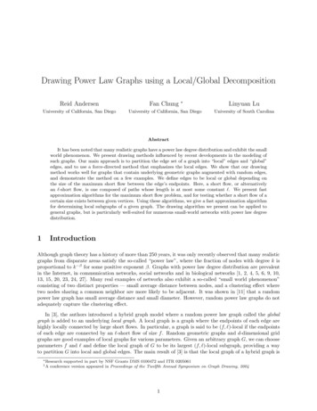
the robustness properties described in Section 2.5. This approach eliminates the recursive part of Extractand requires only M local connectivity tests. It should be considered for large graphs.We remark that for a few limited choices of parameters, testing local connectivity can be solved moreeasily. With the parameters (f 2, ), testing local connectivity can be accomplished by determining thedistance between u and v in G \ (uv). For the parameters (f, 3), testing local connectivity can beaccomplished by computing a maximum bipartite matching.5Applying Local/Global Partitions in Graph DrawingWe combine a local/global partition with a standard force-directed layout method to produce improveddrawings for a variety of graphs. The force-directed method we use is the neato software package fromAT&T [28], which implements a version of the Kamada-Kawai algorithm [21]. Our basic approach is topartition the edge set of the graph into local and global edges, and assign shorter target lengths to localedges. This partitioning method can conceivably be combined with any force-directed layout method whichallows the user to specify either the target lengths or spring constants of edges.To provide motivation, we first demonstrate this approach on a few examples from the hybrid model. Wewill then present a more complicated partition and length assignment rule to be used on real-world examples,and show the results for certain biological networks and collaboration graphs.5.1A Simple Partition and Motivating Examples from the Hybrid ModelHere we demonstrate the application of a straightforward local/global partition to a few idealized examplesfrom the hybrid model. To obtain the results depicted in the figures, we apply the Extract algorithm withappropriate parameters f and to an input graph H to obtain the local subgraph L, and let G H \ L bethe global subgraph. We assign target length 1 to edges in L, and target length 100 to edges in G. In thefigures, the local edges are displayed in a darker color.All the examples described in this section consist of an underlying local graph augmented with randomedges, as in the hybrid model. In all the examples the underlying graph is highly locally connected, and theKamada-Kawai algorithm on its own will produce good drawings of the local graph. However, the KamadaKawai algorithm will not necessarily produce good drawings of the augmented graphs, even though the localgraph may still be easily recoverable from the augmented graph with the Extract algorithm. Combined withour partitioning scheme, the Kamada-Kawai algorithm produces drawings of the augmented graph similarto those of the local graph. This is arguably the best that can be hoped for with a graph from the hybridmodel.The first example is a modified random geometric graph G(n, d, p). A random geometric graph is createdby choosing n points x1 . . . xn uniformly from the unit square, and creating an edge between each pair xi xj ifand only if d(xi , xj ) d. We then augment this graph with the edge set of a random graph G(n, p). We alsoconsider the hypercube Qn and the grid graph Pn Pn augmented with a random graph G(n, p). Note thatQn is an (n, 3)-local graph. The grid graph Pn Pn is a (1, 3)-local graph, and all edges not on the borderare (3, 3)-connected. The infinite grid graph and the toroidal grid graph Cn Cn are (3, 3)-connected. Therandom geometric graph is displayed in the figures below with the local edges displayed in a darker colorthan the global edges. The other examples are included in section 6.10
Figure 2: The modified geometric graph G(n,d,p) withall target lengths equal5.2Figure 3: The same graph with target lengths set bythe Local/Global partition, using (f 3, 3)A More Sophisticated Partition for Real-World ExamplesThe simple local/global partition H [L, G] and length assignment scheme presented in the previous sectionwill not produce good results for real examples. We will present a different partition which attempts toaddress the main problems that arise. Some of the modifications are motivated solely by practical concernsin order to produce reasonable drawings while still incorporating the local/global partition, but many of theobstacles to adapting the local/global partition to real examples are predicted by models of random po
Drawing Power Law Graphs using a Local/Global Decomposition Reid Andersen University of California, San Diego Fan Chung University of California, San Diego Linyuan Lu University of South Carolina Abstract It has been noted that many realistic graphs have a power law de