Transcription
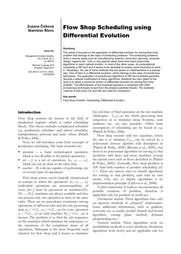
Zuzana ČičkováStanislav ŠtevoArticle Info:Management Information Systems,Vol. 5 (2010), No. 2,pp. 008-013Received 14 January 2010Accepted 2 August 2010UDC 005.311.12:517.9 ; 658.6 ;007:005]:004Flow Shop Scheduling usingDifferential EvolutionSummaryThe article is focused on the application of differential evolution for solving flow shopproblem that belongs to the class of scheduling problems. The scheduling problemsarise in diverse areas such as manufacturing systems, production planning, computerdesign, logistics etc. Only in very special cases there exist exact polynomialalgorithms to reach optimal solution. In most of the other cases, its computationalcomplexity is NP-hard and it seems to be desirable to employ some heuristics to solveit. Nowadays, the use of some methods that are based on metaheuristics is a popularway. One of them is a differential evolution, which belongs to the class of evolutionarytechniques. The application of evolutionary algorithms to NP-hard problems generallyrequires a special modification of these algorithms; therefore the main object of thework is to adapt a canonical version of differential evolution for solving flow shopproblem. The effectiveness of the proposed approach is compared with otherevolutionary techniques known from the already published results. The availableinstance of flow shop Car and Rec are used for comparison.Key wordsFlow Shop Problem, Scheduling, Differential EvolutionIntroductionFlow shop systems are known in the field ofproduction logistics which is called schedulingtheory. This theory includes complicated schedulese.g. production schedules and school schedules,transportation, personal and many others (Palúch& Peško, 2006).Next, we will introduce some basic concepts ofproduction scheduling. The basic elements are: operation – o, basic technological operation,which is not divisible to the partial operations, job – J, is a set of operations {o1, o2, ., on},which can not be done in the same time, machine – M, a device capable of performing oneor several types of operations.Flow shop system can be basically characterizedas systems in which the operations {o1, o2, ., on}(individual operations are uninterruptiblne) ofevery job J must be processed on machines{M1,M2, ., Mm} (machines are always available and theycan process only one operation at time) in the sameorder. There are no precedence constraints amongoperations of different jobs and also the processingtime pij, i 1,2, .n, j 1,2, .m, for every operationoi, i 1,2, .n, on each machine Mj, j 1,2, .m, isknown. The problem is to find the job sequenceson the machines which minimize the makespan, i.e.the maximum of the completion times of alloperations. Makespan is the most frequently usedcriterion for flow shop and it means to minimizethe end time of final operation on the last machine(Makespan - Cmax) so the whole processing time(objectives as to minimize mean flowtime, totalterdiness etc. are also possible). Other basicassumptions of scheduling can be found in e.g.(Palúch & Peško, 2006).Flow shop systems with two machines, wherethe aim is to minimize Cmax, can be solved by apolynomial Johnsons algorithm (full description in(Palúch & Peško, 2006) (Brezina et al., 2009)), butthere is no polynomial algorithm for solving so thatproblems with three and more machines (exceptthe special cases such as those described in (Palúch& Peško, 2006)). Generally, flow shop problem isNP- hard with number of possible schedulling (n!)(m-1). There are various ways to classify algorithmsfor solving so that problem, each with its ownmerits. One way to classify algorithms is byimplementation principle (Čičková et al., 2008):Explicit enumeration. It leads to reconnaissance allpossible solutions of problem, therefore isapplicable only for problem of small size.Deterministic methods. These algorithms base onlyon rigorous methods of „classical” mathematics.Some additional information, such as gradient,convexity etc. is usually needed (branch and boundalgorithm, cutting plane method, dynamicprogramming etc.).Stochastic methods. These algorithms work onprobabilistic methods to solve problems. Stochasticalgorithms work slowly and are applicable only for
Flow Shop Scheduling using Differential Evolution„guessing“ (monte carlo, random search walk,evolutionary computation etc.).Combined methods. Combined methods arecomprised by stochastic and deterministiccomposition. Various metaheuristics algorithm hasbeen devised (ant colony optimization, memeticalgorithms, genetic algorithms etc.). Metaheuristicsconsist of general search procedures whoseprinciples allow them to escape local optimalityusing heuristics design. Evolutionary algorithms aresignificant part of metaheuristics.1. Differential EvolutionDifferential evolution belongs to the class ofevolutionary techniques, where the best knownrepresentatives are genetic algorithms, but there aresome differences e.g. an individual is created withthe use of four parents and it is mutedet two timesetc. The evolutionary algorithms comprise a largenumber of nontraditional computing techniqueswhose common characteristic is that they areinspired by the observation of the nature processes(genetic algorithms, ant colony optimization,differential evolution, etc.), respectively from otherdisciplines (e.g. simulated annealing). Nowadaysevolutionary algorithms are considered to beeffective tools that can be used to search forsolutions of optimization problems. The bigadvantage over traditional methods is that they aredesigned to find global extremes (with built-instochastic component) and that their use does notrequire a priori knowledge of optimized function(convexity, differential etc.).Evolutionary algorithms differ from moretraditional optimization techniques in that theyinvolve a search from a "population" ofindividuals, not from a single one. Each individualrepresents one candidate solution for the givenproblem that is represented by parameters ofindividual. Associated with each individual is alsothe fitness, which represents the relevant value ofobjective function. A population can be viewedas np x d matrix (np - number of individuals in thepopulation, d – number of parameter of individual).Every step involves a competitive selection that iscarried out poor solutions.Differential evolution was introduced by Priceand Storm (Storn & Price, 1997). Differentialevolution, as well as other evolutionary techniques,works well on solving non-constrained problemsthat contain continuous variables, but nowadaysthere were developed few approaches that involvethe solving of constrained problems with integer orbinary variables. Varied approaches were used withmore or less success for solving many realproblems etc. traveling salesman problem, vehiclerouting problem etc. (see (Brezina et al., 2009),(Onwubolu & Babu, 2004), (Palúch & Peško,2006)).The principle of basic verzion of differentialevolution can be described by followingpseudocode:BEGINSETTING of control parameters;INITALIZATION of population;EVALUATION of each individual;WHILE (STOPPING CRITERION is notsatisfied) DOFOR (each individual of the population) DO(REPRODUCTIVE CYCLE):CREATE differential vectorCREATE trial vectorCREATE test vectorIF(EVALUATIONoftestvector) (EVALUATION of current selected individual)THEN (SUBSTITUDE the selected individualwith the test vector)ENDIFENDFORENDWHILEEVALUATE process of calculatingENDThe steps of the algorithm can be brieflysummarized as follows (according to (Zelinka,2002) (Onwubolu & Babu, 2004), where it ispossible to found recommended values fordifferent parameters):Setting of the control parameters. Differentialevolution is controlled by a special set ofparameters. Recommended values for theparameters are usually derived empirically fromexperiments:d – dimensionality. Number of parameters ofindividual (usually also number of arguments ofobjective function).np – population size. Number of individuals inpopulation. recommended setting is 5d to 30d,respectively 100d, in cace the optimized funcion ismultimodal (Zelinka, 2002).g – generations. Represent the maximumnumber of iteration (g is also stopping criterion).cr – crossover constant, cr 0,1 . If the crvalue is set to 0, the mutation test vector is only acopy of the current (fourth) parent. If the cr valueis set to 1, test vector will be created only by threeManagement Information SystemsVol. 5, 2/2010, pp. 008-0139
Zuzana Čičková, Stanislav Števorandomly selected parents and a differentialevolution algorithm is purely stochastic.f– mutation constant, f 0,1 . f specifies thelevel of stochastics in the evolutionary process.Initialization. The population must be initializedat the beginning of evolutionary process. Usuallythe random initialization is used so that eachindividual represents a candidate solution of givenproblem, respectively it can be also used someinformation about the problem (if available). Eachindividual is then evaluated with the fitness (relevantvalue of objective function).The test of stopping condition. In its canonical form,the only stopping criterion is to reach the maximalnumber of iterations (represent by parameter g).Theusermaychangeprogramwith some different type of ending the parameter,eg. stop evolution or reformulate the controlparameters, if over th over the last fixed number ofgenerations has not changed the value of bestindividual and so on.Reproductive cycle. This cycle comprise thecrossing and mutation to create individuals for thenext generation. For each individual xig , i 1,2,.np, from the population another three differentindividuals are chosen (vectors r1, r2, r3). Thedifference of the first two vectors (r1 and r2) givesthe differential vector d, which is multiplied bymutation constant f and added to vector r3. Thus,we get trial vector v. Formally:v x f *( xtjtr 3, jtr 1, jtr 2, j x)(1)j 1, 2., d , t 1, 2., gAfter the mutation process comes theformation of a new individual, which is also calledtest vector xtest so that one element after another isselected from the currently selected individual xigand from the trial vector v and for every pair isgenerated a random number from the interval 0.1 , which is compared with the crossingconstant cr. If the generated random number is lessthan or equal to cr, to the relevant position of xtestcomes the element of trial vector v, otherwise ofcurrent selected individual xig.Formally: xj xr 3 j g f ( xr1 j g xr 2 j g ) , if rand j 0,1 cr j ktest(2)xij g , otherwisewherei 1, 2,., np , j 1, 2,., d , k {1, 2,., d } (3)r1, r 2, r 3 {1, 2,. np} ; r1 r 2 r 3 i10Management Information SystemsVol. 5, 2/2010, pp. 008-013where k is a random index, which always ensures achange of at least one parameter in the test vector.The value of the objective function for the testvector is compared to the value of objectivefunction of the curent selected individual and tothe next generation is selected the vector with thebetter objective value.xtest , ak f cos t (x test ) f cos t (xig ) xig 1 x g , otherwisei(3)So that process continues in each generation forall individuals. The result is a new generation withthe same number of individuals.Evaluation. The whole process of reproductioncontinues until the last (users specified) number ofgenerations is reached. The value of the bestindividualfromeachgenerationis reflected to history vector, which shows theprogression of an evolutionary process.2. Flow shop problem usingdifferential evolutionSince the differential evolution is an algorithm,which works well in the case of non-constrainedproblems with continuous variables, in applying thealgorithm for solving NP-hard problems, isnecessary to consider the following factors: Selection of an appropriate representation ofindividual Formulation of objective function Transformation the parameters of individual tothe real numbers Transformation of unfeasible solutions Setting of the control parameters of thedifferential evolutionSelection of an appropriate representation of individual.A natural representation of individual, that isparticularly known from genetic algorithms (wherehas been often used with success by solving muchknown traveling salesman problem), was chosen.In response to the flow shop problem, eachoperation is assigned with integer from 1 to n (nrepresents the number of operations), whichrepresents corresponding operation in individual.Each individual is then represented by a ddimensional vector of integers, representing directthe order of processing operations. Then, the initialpopulation is generated as follows:( )( )P x randperm ( d )i, j00i 1, 2,., np j 1, 2,., d (4)
Flow Shop Scheduling using Differential Evolutionwhere the function randperm (d) ensure theestablishment of a random permutation of dintegers, so it is the random permutation of thesequence of operations. Each individual in thepopulation is also assigned with its fitness thatrepresents maximum of the completion times of alloperations (Makespan).Formulation of objective function. The computationof objective function value for an individual iscarried out in two steps with respect the followingfacts:1. The first machine begins to process the firstoperation in sequence in time 0 and thisoperation will not proceed on the next machineunless its processing on first machine is done.2. Processing of other operations in the sequenceis as follows: the first machine works without downtime, i.e.operations are assigned in the order, which isdetermined by individual the processing of relevant operation on thefurther machines is conditioned by fact that themachine is already free (if not, relevantoperation waits for completion of previousoperation on this machine) and also the processing of relevant operationtasks on the previous machine is done (ifno, there is a machine downtime, waiting forthe operation).Transformation the parameters of individual to the realnumbers. Because the differential evolutionalgorithm was originally designed to solveproblems with continuous-time variables and theused natural representation consists of integervariables, it is desirable to transform integers to realnumbers. The used method for transformation waspresented in (Onwubolu & Babu, 2004) for solvingtraveling salesman problem. Let zi, i 1, 2, .,nrepresents an integer number. The equivalentcontinuous variable for zi is given as:z * f *5ri 1 i 310 1where f is given, for example. f 200.zi 5* f α int ( zi 0,5 )(8)Transformation of unfeasible solutions. The use ofdifferential evolution algorithm does not requirethe formation of feasible solution in case of naturalrepresentation of individual, therefore it isnecessary to choose an appropriate method oftransformation of the unfeasible solutions. Theproblem of infeasibility occurs in two cases:a) Parameter of individual after the transformationfrom real numbers to integers is less then 1 orgreater then d, in this case the relevantparameter is replaced by new randomlygenerated parameters in range 1 to d.b) Created individual does not comprise apermutation of integers d. In this case, thecorrection approach that was presented in(Brezina et al, 2009) by solving vehicle routingproblem, was used.1) Let m is the vector of parameters of theindividual dimension of d with k differentelements. If d - k 0, go to step 4). Otherwise,go to step 2).2) Create the vector p (dimension d - k) of randompermutation of such d – k elements,which are not included in the vector m. If thenumber of non-zero components of the vectorp 0, go to step 4). Otherwise, find the firstrepeated element of vector m. Let this elementbe mc and let the first nonzero element of vectorp be pk . Set mc pk and go to step 3).3) Set pk 0 and return to the step 2).4) Return mAs part of the software support for experimens,the MATLAB 7.1 was used. Two functions werecreated: the differential evolution algorithmadapted for solving flow shop systems and thefunction for objective function calculation thatcalculates the value of optimized function.3. Experiments(6)To discover the effectiveness of the presentedtechniques, the free available test data Car1 up to1Car8 from OR library were used. This Flow shopinstances were investigated by many researcherswho applied a variety of techniques to solve it (andalso there is a known optimal value of objectivefunction). Firstly, the 165 simulation were carriedout to determine the effective setting of control(7)1(5)Reverse transformation of real numbers to integers(used to evaluate the objective function):(1 ri ) * (103 1)β α zihttp://people.brunel.ac.uk/ mastjjb/jeb/orlib/files/(15.9.2010)Management Information SystemsVol. 5, 2/2010, pp. 008-01311
Zuzana Čičková, Stanislav Števoparameters f and cr (with the simultanous use of theset np 300, g 1500). The best parametersobtained from combining these parameters duringexperimentation are: cr 0,1 and f 0,05. Altroghtthose setting presents a relative low crossing rateand mutation, they seemed to be adequate togarantee evolution process. After all simulation wecan resume that we were able to achive optimalsolution for all instances Car.Further on, the test data Rec 03 up to Rec 17also from OR library were solved with the use ofcontrol parameters: cr 0,1, f 0,05, np 300, g 4500 and the test data Rec 19 up to Rec 29 withthe use of control parameters: cr 0,1, f 0,05, np 500, g 8500. For each problem threesimulations were done. The results are given inTable 1:Table 1 Results for Rec instancesProblem Size 1112Simulation2 Simulation3 Mean 5In order to compare the before mentionedapproach with other minimizing strategies thework (Davendra & Zelinka, 2008) was used. Therewere published the results of following fiveevolutionary algorithms:H-GA – Hybrid Genetic AlgorithmOGA – Othogonal Genetic AlgorithmIGA – Improved Genetic Algorithm2First number represents the number of operations, secondnumber represents the number of machines.12Management Information SystemsVol. 5, 2/2010, pp. 008-013MAEA – Multiagent Evolutionary AlgorithmSOMA – Self Organizing Migrating AlgorithmThe compatrision of differential evolution withthese evolutionary approaches is given in Table 2,where the percentage deviations from optimalvalue for different evolutionary techniques areseen.Table 2 Comparison with other 731,182,090,80,560,011,56From the last column of Table 2 it is evidentthat the percentage deviation of results obtained bydifferential evolution algorithm from the optimalsolution was less than 1.7%. The results for theinstance Car are consistent with the optimalsolution in every case. Problems Rec01 up toRec17 were solved with the percentage deviationfrom optimal value within the range from 0 to0.56% and problems Rec19 up to Rec29 within therange from 0.91 to 1.67%.Based on these results it can be stated that thedifferential evolution presents a powerfullapproach for solving flow shop problems. To dealwith the number of operations less than 20, theoptimal solution was obtained in every case, in thecase of sequencing of 20 operacions, thepercentage deviations from the optimal solutionwere less than 1% and in case of sequencing of 30operations the percentage deviations from theoptimal solution were always less than 1.7%. As itis seen from the Table 2, presented approach isfully comparable with the published results ofother evolutionary techniques.
Flow Shop Scheduling using Differential EvolutionConclusionFlow shop problem is one of NP-hard problems. Atypical conflict in dealing with this kind ofproblems arises between the time available for thecalculation and the quality of the solution. Whilethe exact methods (eg, branch and boundalgorithm) are often able to identify the optimumin unacceptably long time, the quality of solutionsobtained by heuristic may be disputable.Nowadays, we follow the increased interest inmethods, which are inspired by different biologicalevolutionary processes in nature. This technologyis covered by the common name of "evolutionaryalgorithms". But their application to constrainedproblems requires some additional modifications oftheirs basic versions. The paper was focused onapplication of differential evolution to flow shopproblem. The special factors that involve the use ofdifferential evolution were presented and theefficiency of calculations has been validated on thebasis of publicly available instances. Based onpresented results it can be concluded that theproposed approach is quite powerful in dealingwith flow shop problem and it is fully comparablewith the published results of other evolutionarytechniques.Zuzana ČičkováUniversity of Economics in BratislavaDepartment of Operations Research and Econometrics, Faculty ofEconomic InformaticsDolnozemská cesta 1/b852 35 BratislavaSlovak RepublicEmail: cickova@euba.skReferencesBrezina, I., Čičková, Z., & Reiff, M. (2009). Kvantitatívnemetódy na podporu logistických procesov. Bratislava:Ekonóm.Brezina, I., Čičková, Z., Gežik, P., & Pekár, J. (2009).Modelovanie reverznej logistiky – optimalizácia procesovrecyklácie a likvidácie odpadu. Bratislava: Ekonóm.Čičková, Z., Brezina, I., & Pekár, P. (2008). Alternativemethod for solving traveling salesman problem byevolutionary algorithm. Management information systems , 3(1), 17-22.Davendra, D., & Zelinka, I. (2008). Flow Shop Schedulingusing Self Organizing migration Algorithm. 22nd EuropeanConference on Modelling and Simulation, (pp. 195-200).Nicosia.Onwubolu, G., & Babu, B. (2004). New OptimizationTechniques in Engineering, Studies in Fuzziness and SoftComputing. New York: Springer.Paluch, S., & Peško, Š. (2006). Kvantitatívne metódy vlogistike. Žilina: EDIS vydavateľstvo ŽU.Sekaj, I. (2005). Evolučné výpočty a ich využitie v praxi.Bratislava: IRIS.Storn, R., & Price, K. (1997). Differential Evolution – a simpleand efficient heuristic for global optimization over continuousspaces. Jounal of Global Optimization , 11 (4), 341-359.Zelinka, I. (2002). Umělá inteligence v problémech globálníoptimalizace. Praha: BEN-technická literatúra.Stanislav ŠtevoSlovak University of TechnologyInstitute of Control and Industrial Informatics, Faculty of ElectricalEngineering and Information TechnologyIlkovičova 3852 35 BratislavaSlovak RepublicEmail: stanislav.stevo@stuba.skManagement Information SystemsVol. 5, 2/2010, pp. 008-01313
Flow shop systems are known in the field of production logistics which scheduling is called theory. This theory includes complicated schedules e.g. production schedules and school schedules, transportation, personal and many others (Palúch & Peško, 2006). Next, we will introduce some basic concepts of production scheduling. The basic elements .