Transcription
Partial Differential EquationsLecture NotesErich MiersemannDepartment of MathematicsLeipzig UniversityVersion October, 2012
2
Contents1 Introduction1.1 Examples . . . . . . . . . . . . . . . .1.2 Equations from variational problems .1.2.1 Ordinary differential equations1.2.2 Partial differential equations .1.3 Exercises . . . . . . . . . . . . . . . .2 Equations of first order2.1 Linear equations . . . . . . . . . . . .2.2 Quasilinear equations . . . . . . . . .2.2.1 A linearization method . . . .2.2.2 Initial value problem of Cauchy2.3 Nonlinear equations in two variables .2.3.1 Initial value problem of Cauchy2.4 Nonlinear equations in Rn . . . . . . .2.5 Hamilton-Jacobi theory . . . . . . . .2.6 Exercises . . . . . . . . . . . . . . . .91115151622.252531323340485153593 Classification3.1 Linear equations of second order . . . . .3.1.1 Normal form in two variables . . .3.2 Quasilinear equations of second order . . .3.2.1 Quasilinear elliptic equations . . .3.3 Systems of first order . . . . . . . . . . . .3.3.1 Examples . . . . . . . . . . . . . .3.4 Systems of second order . . . . . . . . . .3.4.1 Examples . . . . . . . . . . . . . .3.5 Theorem of Cauchy-Kovalevskaya . . . . .3.5.1 Appendix: Real analytic functions.63636973737476828384903.
4CONTENTS3.6Exercises. . . . . . . . . . . . . . . . . . . . . . . . . . . . . 1014 Hyperbolic equations4.1 One-dimensional wave equation . . . . .4.2 Higher dimensions . . . . . . . . . . . .4.2.1 Case n 3 . . . . . . . . . . . . .4.2.2 Case n 2 . . . . . . . . . . . .4.3 Inhomogeneous equation . . . . . . . . .4.4 A method of Riemann . . . . . . . . . .4.5 Initial-boundary value problems . . . . .4.5.1 Oscillation of a string . . . . . .4.5.2 Oscillation of a membrane . . . .4.5.3 Inhomogeneous wave equations .4.6 Exercises . . . . . . . . . . . . . . . . .107. 107. 109. 112. 115. 117. 120. 125. 125. 128. 131. 1365 Fourier transform1415.1 Definition, properties . . . . . . . . . . . . . . . . . . . . . . . 1415.1.1 Pseudodifferential operators . . . . . . . . . . . . . . . 1465.2 Exercises . . . . . . . . . . . . . . . . . . . . . . . . . . . . . 1496 Parabolic equations6.1 Poisson’s formula . . . . . . . .6.2 Inhomogeneous heat equation .6.3 Maximum principle . . . . . . .6.4 Initial-boundary value problem6.4.1 Fourier’s method . . . .6.4.2 Uniqueness . . . . . . .6.5 Black-Scholes equation . . . . .6.6 Exercises . . . . . . . . . . . .7 Elliptic equations of second order7.1 Fundamental solution . . . . . . . . . . . . . . . . .7.2 Representation formula . . . . . . . . . . . . . . . .7.2.1 Conclusions from the representation formula7.3 Boundary value problems . . . . . . . . . . . . . . .7.3.1 Dirichlet problem . . . . . . . . . . . . . . . .7.3.2 Neumann problem . . . . . . . . . . . . . . .7.3.3 Mixed boundary value problem . . . . . . . .7.4 Green’s function for 4 . . . . . . . . . . . . . . . . .7.4.1 Green’s function for a ball . . . . . . . . . . .151. 152. 155. 156. 162. 162. 164. 164. 170.175. 175. 177. 179. 181. 181. 182. 183. 183. 186
CONTENTS7.57.657.4.2 Green’s function and conformal mapping . . . . . . . 190Inhomogeneous equation . . . . . . . . . . . . . . . . . . . . . 190Exercises . . . . . . . . . . . . . . . . . . . . . . . . . . . . . 195
6CONTENTS
PrefaceThese lecture notes are intented as a straightforward introduction to partialdifferential equations which can serve as a textbook for undergraduate andbeginning graduate students.For additional reading we recommend following books: W. I. Smirnov [21],I. G. Petrowski [17], P. R. Garabedian [8], W. A. Strauss [23], F. John [10],L. C. Evans [5] and R. Courant and D. Hilbert[4] and D. Gilbarg and N. S.Trudinger [9]. Some material of these lecture notes was taken from some ofthese books.7
8CONTENTS
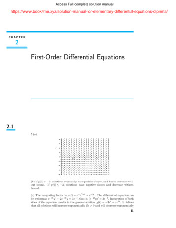
Chapter 1IntroductionOrdinary and partial differential equations occur in many applications. Anordinary differential equation is a special case of a partial differential equation but the behaviour of solutions is quite different in general. It is muchmore complicated in the case of partial differential equations caused by thefact that the functions for which we are looking at are functions of morethan one independent variable.EquationF (x, y(x), y 0 (x), . . . , y (n) ) 0is an ordinary differential equation of n-th order for the unknown functiony(x), where F is given.An important problem for ordinary differential equations is the initialvalue problemy 0 (x) f (x, y(x))y(x0 ) y0 ,where f is a given real function of two variables x, y and x0 , y0 are givenreal numbers.Picard-Lindelöf Theorem. Suppose(i) f (x, y) is continuous in a rectangleQ {(x, y) R2 : x x0 a, y y0 b}.(ii) There is a constant K such that f (x, y) K for all (x, y) Q.(ii) Lipschitz condition: There is a constant L such that f (x, y2 ) f (x, y1 ) L y2 y1 9
10CHAPTER 1. INTRODUCTIONyy0x0xFigure 1.1: Initial value problemfor all (x, y1 ), (x, y2 ).Then there exists a unique solution y C 1 (x0 α, x0 α) of the above initialvalue problem, where α min(b/K, a).The linear ordinary differential equationy (n) an 1 (x)y (n 1) . . . a1 (x)y 0 a0 (x)y 0,where aj are continuous functions, has exactly n linearly independent solutions. In contrast to this property the partial differential uxx uyy 0 in R2has infinitely many linearly independent solutions in the linear space C 2 (R2 ).The ordinary differential equation of second ordery 00 (x) f (x, y(x), y 0 (x))has in general a family of solutions with two free parameters. Thus, it isnaturally to consider the associated initial value problemy 00 (x) f (x, y(x), y 0 (x))y(x0 ) y0 , y 0 (x0 ) y1 ,where y0 and y1 are given, or to consider the boundary value problemy 00 (x) f (x, y(x), y 0 (x))y(x0 ) y0 , y(x1 ) y1 .Initial and boundary value problems play an important role also in thetheory of partial differential equations. A partial differential equation for
111.1. EXAMPLESyy1y0x0x1xFigure 1.2: Boundary value problemthe unknown function u(x, y) is for exampleF (x, y, u, ux , uy , uxx , uxy , uyy ) 0,where the function F is given. This equation is of second order.An equation is said to be of n-th order if the highest derivative whichoccurs is of order n.An equation is said to be linear if the unknown function and its derivatives are linear in F . For example,a(x, y)ux b(x, y)uy c(x, y)u f (x, y),where the functions a, b, c and f are given, is a linear equation of firstorder.An equation is said to be quasilinear if it is linear in the highest derivatives. For example,a(x, y, u, ux , uy )uxx b(x, y, u, ux , uy )uxy c(x, y, u, ux , uy )uyy 0is a quasilinear equation of second order.1.1Examples1. uy 0, where u u(x, y). All functions u w(x) are solutions.2. ux uy , where u u(x, y). A change of coordinates transforms thisequation into an equation of the first example. Set ξ x y, η x y,then¶µξ η ξ η, : v(ξ, η).u(x, y) u22
12CHAPTER 1. INTRODUCTIONAssume u C 1 , then1vη (ux uy ).2If ux uy , then vη 0 and vice versa, thus v w(ξ) are solutions forarbitrary C 1 -functions w(ξ). Consequently, we have a large class of solutionsof the original partial differential equation: u w(x y) with an arbitraryC 1 -function w.3. A necessary and sufficient condition such that for given C 1 -functionsM, N the integralZ P1M (x, y)dx N (x, y)dyP0is independent of the curve which connects the points P0 with P1 in a simplyconnected domain Ω R2 is the partial differential equation (condition ofintegrability)My N xin Ω.ΩyP1P0xFigure 1.3: Independence of the pathThis is one equation for two functions. A large class of solutions is givenby M Φx , N Φy , where Φ(x, y) is an arbitrary C 2 -function. It followsfrom Gauss theorem that these are all C 1 -solutions of the above differentialequation.4. Method of an integrating multiplier for an ordinary differential equation.Consider the ordinary differential equationM (x, y)dx N (x, y)dy 0
131.1. EXAMPLESfor given C 1 -functions M, N . Then we seek a C 1 -function µ(x, y) such thatµM dx µN dy is a total differential, i. e., that (µM )y (µN )x is satisfied.This is a linear partial differential equation of first order for µ:M µy N µx µ(Nx My ).5. Two C 1 -functions u(x, y) and v(x, y) are said to be functionally dependentif¶µux uy 0,detvx vywhich is a linear partial differential equation of first order for u if v is a givenC 1 -function. A large class of solutions is given byu H(v(x, y)),where H is an arbitrary C 1 -function.6. Cauchy-Riemann equations. Set f (z) u(x, y) iv(x, y), where z x iyand u, v are given C 1 (Ω)-functions. Here is Ω a domain in R2 . If the functionf (z) is differentiable with respect to the complex variable z then u, v satisfythe Cauchy-Riemann equationsux vy , uy vx .It is known from the theory of functions of one complex variable that thereal part u and the imaginary part v of a differentiable function f (z) aresolutions of the Laplace equation4u 0, 4v 0,where 4u uxx uyy .7. The Newton potentialu p1x2 y 2 z 2is a solution of the Laplace equation in R3 \ (0, 0, 0), i. e., ofuxx uyy uzz 0.
14CHAPTER 1. INTRODUCTION8. Heat equation. Let u(x, t) be the temperature of a point x Ω at timet, where Ω R3 is a domain. Then u(x, t) satisfies in Ω [0, ) the heatequationut k4u,where 4u ux1 x1 ux2 x2 ux3 x3 and k is a positive constant. The conditionu(x, 0) u0 (x), x Ω,where u0 (x) is given, is an initial condition associated to the above heatequation. The conditionu(x, t) h(x, t), x Ω, t 0,where h(x, t) is given is a boundary condition for the heat equation.If h(x, t) g(x), that is, h is independent of t, then one expects that thesolution u(x, t) tends to a function v(x) if t . Moreover, it turns outthat v is the solution of the boundary value problem for the Laplace equation4v 0 in Ωv g(x) on Ω.9. Wave equation. The wave equationyu(x,t 1)u(x,t 2)lxFigure 1.4: Oscillating stringutt c2 4u,where u u(x, t), c is a positive constant, describes oscillations of membranes or of three dimensional domains, for example. In the one-dimensionalcaseutt c2 uxxdescribes oscillations of a string.
1.2. EQUATIONS FROM VARIATIONAL PROBLEMS15Associated initial conditions areu(x, 0) u0 (x), ut (x, 0) u1 (x),where u0 , u1 are given functions. Thus the initial position and the initialvelocity are prescribed.If the string is finite one describes additionally boundary conditions, forexampleu(0, t) 0, u(l, t) 0 for all t 0.1.2Equations from variational problemsA large class of ordinary and partial differential equations arise from variational problems.1.2.1Ordinary differential equationsSetE(v) Zbf (x, v(x), v 0 (x)) dxaand for given ua , ub RV {v C 2 [a, b] : v(a) ua , v(b) ub },where a b and f is sufficiently regular. One of the basicproblems in the calculus of variation is(P )minv V E(v).Euler equation. Let u V be a solution of (P), thendfu0 (x, u(x), u0 (x)) fu (x, u(x), u0 (x))dxin (a, b).Proof. Exercise. Hints: For fixed φ C 2 [a, b] with φ(a) φ(b) 0 andreal ², ² ²0 , set g(²) E(u ²φ). Since g(0) g(²) it follows g 0 (0) 0.Integration by parts in the formula for g 0 (0) and the following basic lemmain the calculus of variations imply Euler’s equation.
16CHAPTER 1. INTRODUCTIONyy1y0abxFigure 1.5: Admissible variationsBasic lemma in the calculus of variations. Let h C(a, b) andZ bh(x)φ(x) dx 0afor all φ C01 (a, b). Then h(x) 0 on (a, b).Proof. Assume h(x0 ) 0 for an x0 (a, b), then there is a δ 0 such that(x0 δ, x0 δ) (a, b) and h(x) h(x0 )/2 on (x0 δ, x0 δ). Set½ ¡ 2δ 2 x x0 2if x (x0 δ, x0 δ)φ(x) .0 if x (a, b) \ [x0 δ, x0 δ]Thus φ C01 (a, b) andZZ bh(x0 ) x0 δφ(x) dx 0,h(x)φ(x) dx 2x0 δawhich is a contradiction to the assumption of the lemma.1.2.22Partial differential equationsThe same procedure as above applied to the following multiple integral leadsto a second-order quasilinear partial differential equation. SetZE(v) F (x, v, v) dx,Ω
1.2. EQUATIONS FROM VARIATIONAL PROBLEMS17where Ω Rn is a domain, x (x1 , . . . , xn ), v v(x) : Ω 7 R, and v (vx1 , . . . , vxn ). Assume that the function F is sufficiently regular inits arguments. For a given function h, defined on Ω, setV {v C 2 (Ω) : v h on Ω}.Euler equation. Let u V be a solution of (P), thennX Fu Fu 0 xi xii 1in Ω.Proof. Exercise. Hint: Extend the above fundamental lemma of the calculusof variations to the case of multiple integrals. The interval (x0 δ, x0 δ) inthe definition of φ must be replaced by a ball with center at x0 and radiusδ.Example: Dirichlet integralIn two dimensions the Dirichlet integral is given byZ¡ 2 D(v) vx vy2 dxdyΩand the associated Euler equation is the Laplace equation 4u 0 in Ω.Thus, there is natural relationship between the boundary value problem4u 0 in Ω, u h on Ωand the variational problemmin D(v).v VBut these problems are not equivalent in general. It can happen that theboundary value problem has a solution but the variational problem has nosolution, see for an example Courant and Hilbert [4], Vol. 1, p. 155, whereh is a continuous function and the associated solution u of the boundaryvalue problem has no finite Dirichlet integral.The problems are equivalent, provided the given boundary value functionh is in the class H 1/2 ( Ω), see Lions and Magenes [14].
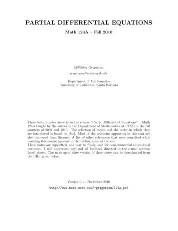
18CHAPTER 1. INTRODUCTIONExample: Minimal surface equationThe non-parametric minimal surface problem in two dimensions is tofind a minimizer u u(x1 , x2 ) of the problemZ qmin1 vx21 vx22 dx,v VΩwhere for a given function h defined on the boundary of the domain ΩV {v C 1 (Ω) : v h on Ω}.SΩFigure 1.6: Comparison surfaceSuppose that the minimizer satisfies the regularity assumption u C 2 (Ω),then u is a solution of the minimal surface equation (Euler equation) in Ω!ÃÃ! u x1u x2pp 0.(1.1) x1 x21 u 21 u 2In fact, the additional assumption u C 2 (Ω) is superfluous since it followsfrom regularity considerations for quasilinear elliptic equations of secondorder, see for example Gilbarg and Trudinger [9].Let Ω R2 . Each linear function is a solution of the minimal surfaceequation (1.1). It was shown by Bernstein [2] that there are no other solutions of the minimal surface quation. This is true also for higher dimensions
1.2. EQUATIONS FROM VARIATIONAL PROBLEMS19n 7, see Simons [19]. If n 8, then there exists also other solutions whichdefine cones, see Bombieri, De Giorgi and Giusti [3].The linearized minimal surface equation over u 0 is the Laplace equation 4u 0. In R2 linear functions are solutions but also many otherfunctions in contrast to the minimal surface equation. This striking difference is caused by the strong nonlinearity of the minimal surface equation.More general minimal surfaces are described by using parametric representations. An example is shown in Figure 1.71 . See [18], pp. 62, forexample, for rotationally symmetric minimal surfaces.Figure 1.7: Rotationally symmetric minimal surfaceNeumann type boundary value problemsSet V C 1 (Ω) andE(v) ZΩF (x, v, v) dx Zg(x, v) ds, Ωwhere F and g are given sufficiently regular functions and Ω Rn is abounded and sufficiently regular domain. Assume u is a minimizer of E(v)in V , that isu V : E(u) E(v) for all v V,1An experiment from Beutelspacher’s Mathematikum, Wissenschaftsjahr 2008, Leipzig
20CHAPTER 1. INTRODUCTIONthenZΩn¡Xi 1Fuxi (x, u, u)φxi Fu (x, u, u)φ dx Zgu (x, u)φ ds 0 Ωfor all φ C 1 (Ω). Assume additionally u C 2 (Ω), then u is a solution ofthe Neumann type boundary value problemnX Fu Fu 0 in Ω xi xii 1nXi 1Fuxi νi gu 0 on Ω,where ν (ν1 , . . . , νn ) is the exterior unit normal at the boundary Ω. Thisfollows after integration by parts from the basic lemma of the calculus ofvariations.Example: Laplace equationSet1E(v) 2ZΩ2 v dx Zh(x)v ds, Ωthen the associated boundary value problem is4u 0 in Ω u h on Ω. νExample: Capillary equationLet Ω R2 and setZZZ pκ22v ds.v dx cos γ1 v dx E(v) 2 Ω ΩΩHere κ is a positive constant (capillarity constant) and γ is the (constant)boundary contact angle, i. e., the angle between the container wall and
1.2. EQUATIONS FROM VARIATIONAL PROBLEMS21the capillary surface, defined by v v(x1 , x2 ), at the boundary. Then therelated boundary value problem isdiv (T u) κu in Ων · T u cos γ on Ω,where we use the abbreviation uTu p,1 u 2div (T u) is the left hand side of the minimal surface equation (1.1) and itis twice the mean curvature of the surface defined by z u(x1 , x2 ), see anexercise.The above problem describes the ascent of a liquid, water for example,in a vertical cylinder with cross section Ω. Assume the gravity is directeddownwards in the direction of the negative x3 -axis. Figure 1.8 shows thatliquid can rise along a vertical wedge which is a consequence of the strongnonlinearity of the underlying equations, see Finn [7]. This photo was takenFigure 1.8: Ascent of liquid in a wedgefrom [15].
22CHAPTER 1. INTRODUCTION1.3Exercises1. Find nontrivial solutions u ofux y u y x 0 .2. Prove: In the linear space C 2 (R2 ) there are infinitely many linearlyindependent solutions of 4u 0 in R2 .Hint: Real and imaginary part of holomorphic functions are solutionsof the Laplace equation.3. Find all radially symmetric functions which satisfy the Laplace equation in Rn \{0} for n 2. APfunction u is said to be radially symmetricif u(x) f (r), where r ( ni x2i )1/2 .¡ 0Hint: Show that a radially symmetric u satisfies 4u r1 n rn 1 f 0by using u(x) f 0 (r) xr .4. Prove the basic lemma in the calculus of variations: Let Ω Rn be adomain and f C(Ω) such thatZf (x)h(x) dx 0Ωfor all h C02 (Ω). Then f 0 in Ω.5. Write the minimal surface equation (1.1) as a quasilinear equation ofsecond order.6. Prove that a sufficiently regular minimizer in C 1 (Ω) ofZZE(v) F (x, v, v) dx g(v, v) ds,Ω Ωis a solution of the boundary value problemnX Fu Fu 0 in Ω xi xii 1nXi 1Fuxi νi gu 0 on Ω,where ν (ν1 , . . . , νn ) is the exterior unit normal at the boundary Ω.
231.3. EXERCISES7. Prove that ν · T u cos γ on Ω, where γ is the angle between thecontainer wall, which is here a cylinder, and the surface S, defined byz u(x1 , x2 ), at the boundary of S, ν is the exterior normal at Ω.Hint: The angle between two surfaces is by definition the angle betweenthe two associated normals at the intersection of the surfaces.8. Let Ω be bounded and assume u C 2 (Ω) is a solution ofdiv T u C in Ω uν·p cos γ on Ω,1 u 2where C is a constant.Prove thatC Ω cos γ . Ω Hint: Integrate the differential equation over Ω.9. Assume Ω BR (0) is a disc with radius R and the center at pthe origin.Show that radially symmetric solutions u(x) w(r), r x21 x22 ,of the capillary boundary value problem are solutions ofµ¶0rw0 κrw in 0 r R1 w02w0 cos γ if r R.1 w02Remark. It follows from a maximum principle of Concus and Finn [7]that a solution of the capillary equation over a disc must be radiallysymmetric.10. Find all radially symmetric solutions of¶0µrw0 Cr in 0 r R1 w02w0 cos γ if r R.1 w02Hint: From an exercise above it follows that2C cos γ.R
24CHAPTER 1. INTRODUCTION11. Show that div T u is twice the mean curvature of the surface definedby z u(x1 , x2 ).
Chapter 2Equations of first orderFor a given sufficiently regular function F the general equation of first orderfor the unknown function u(x) isF (x, u, u) 0in Ω Rn . The main tool for studying related problems is the theory ofordinary differential equations. This is quite different for systems of partialdifferential of first order.The general linear partial differential equation of first order can be written asnXai (x)uxi c(x)u f (x)i 1for given functions ai , c and f . The general quasilinear partial differentialequation of first order isnXai (x, u)uxi c(x, u) 0.i 12.1Linear equationsLet us begin with the linear homogeneous equationa1 (x, y)ux a2 (x, y)uy 0.(2.1)Assume there is a C 1 -solution z u(x, y). This function defines a surfaceS which has at P (x, y, u(x, y)) the normal1N p( ux , uy , 1)1 u 225
26CHAPTER 2. EQUATIONS OF FIRST ORDERand the tangential plane defined byζ z ux (x, y)(ξ x) uy (x, y)(η y).Set p ux (x, y), q uy (x, y) and z u(x, y). The tuple (x, y, z, p, q) iscalled surface element and the tuple (x, y, z) support of the surface element.The tangential plane is defined by the surface element. On the other hand,differential equation (2.1)a1 (x, y)p a2 (x, y)q 0defines at each support (x, y, z) a bundle of planes if we consider all (p, q) satisfying this equation. For fixed (x, y), this family of planes Π(λ) Π(λ; x, y)is defined by a one parameter family of ascents p(λ) p(λ; x, y), q(λ) q(λ; x, y). The envelope of these planes is a line sincea1 (x, y)p(λ) a2 (x, y)q(λ) 0,which implies that the normal N(λ) on Π(λ) is perpendicular on (a1 , a2 , 0).Consider a curve x(τ ) (x(τ ), y(τ ), z(τ )) on S, let Tx0 be the tangentialplane at x0 (x(τ0 ), y(τ0 ), z(τ0 )) of S and consider on Tx0 the lineL : l(σ) x0 σx0 (τ0 ), σ R,see Figure 2.1.We assume L coincides with the envelope, which is a line here, of thefamily of planes Π(λ) at (x, y, z). Assume that Tx0 Π(λ0 ) and considertwo planesΠ(λ0 ) :Π(λ0 h) :z z0 (x x0 )p(λ0 ) (y y0 )q(λ0 )z z0 (x x0 )p(λ0 h) (y y0 )q(λ0 h).At the intersection l(σ) we have(x x0 )p(λ0 ) (y y0 )q(λ0 ) (x x0 )p(λ0 h) (y y0 )q(λ0 h).Thus,x0 (τ0 )p0 (λ0 ) y 0 (τ0 )q 0 (λ0 ) 0.From the differential equationa1 (x(τ0 ), y(τ0 ))p(λ) a2 (x(τ0 ), y(τ0 ))q(λ) 0
272.1. LINEAR EQUATIONSzLΠ( λ 0 )ySxFigure 2.1: Curve on a surfaceit followsa1 p0 (λ0 ) a2 q 0 (λ0 ) 0.Consequently(x0 (τ ), y 0 (τ )) x0 (τ )(a1 (x(τ ), y(τ )), a2 (x(τ ), y(τ )),a1 (x(τ, y(τ ))since τ0 was an arbitrary parameter. Here we assume that x0 (τ ) 6 0 anda1 (x(τ ), y(τ )) 6 0.Then we introduce a new parameter t by the inverse of τ τ (t), whereZ τx0 (s)ds.t(τ ) τ0 a1 (x(s), y(s))It follows x0 (t) a1 (x, y), y 0 (t) a2 (x, y). We denote x(τ (t)) by x(t) again.Now we consider the initial value problemx0 (t) a1 (x, y), y 0 (t) a2 (x, y), x(0) x0 , y(0) y0 .(2.2)From the theory of ordinary differential equations it follows (Theorem ofPicard-Lindelöf) that there is a unique solution in a neighbouhood of t 0provided the functions a1 , a2 are in C 1 . From this definition of the curves
28CHAPTER 2. EQUATIONS OF FIRST ORDER(x(t), y(t)) is follows that the field of directions (a1 (x0 , y0 ), a2 (x0 , y0 )) definesthe slope of these curves at (x(0), y(0)).Definition. The differential equations in (2.2) are called characteristicequations or characteristic system and solutions of the associated initial valueproblem are called characteristic curves.Definition. A function φ(x, y) is said to be an integral of the characteristicsystem if φ(x(t), y(t)) const. for each characteristic curve. The constantdepends on the characteristic curve considered.Proposition 2.1. Assume φ C 1 is an integral, then u φ(x, y) is asolution of (2.1).Proof. Consider for given (x0 , y0 ) the above initial value problem (2.2).Since φ(x(t), y(t)) const. it followsφx x0 φy y 0 0for t t0 , t0 0 and sufficiently small. Thusφx (x0 , y0 )a1 (x0 , y0 ) φy (x0 , y0 )a2 (x0 , y0 ) 0.2Remark. If φ(x, y) is a solution of equation (2.1) then also H(φ(x, y)),where H(s) is a given C 1 -function.Examples1. Considera1 ux a2 uy 0,where a1 , a2 are constants. The system of characteristic equations isx0 a1 , y 0 a2 .Thus the characteristic curves are parallel straight lines defined byx a1 t A, y a2 t B,
292.1. LINEAR EQUATIONSwhere A, B are arbitrary constants. From these equations it follows thatφ(x, y) : a2 x a1 yis constant along each characteristic curve. Consequently, see Proposition 2.1, u a2 x a1 y is a solution of the differential equation. Froman exercise it follows thatu H(a2 x a1 y),(2.3)where H(s) is an arbitrary C 1 -function, is also a solution. Since u is constantwhen a2 x a1 y is constant, equation (2.3) defines cylinder surfaces whichare generated by parallel straight lines which are parallel to the (x, y)-plane,see Figure 2.2.zyxFigure 2.2: Cylinder surfaces2. Consider the differential equationxux yuy 0.The characteristic equations arex0 x, y 0 y,
30CHAPTER 2. EQUATIONS OF FIRST ORDERand the characteristic curves are given byx Aet , y Bet ,where A, B are arbitrary constants. Thus, an integral is y/x, x 6 0, and fora given C 1 -function the function u H(x/y) is a solution of the differentialequation. If y/x const., then u is constant. Suppose that H 0 (s) 0,for example, then u defines right helicoids (in German: Wendelflächen), seeFigure 2.3Figure 2.3: Right helicoid, a2 x2 y 2 R2 (Museo Ideale Leonardo daVinci, Italy)3. Consider the differential equationyux xuy 0.The associated characteristic system isx0 y, y 0 x.If followsx0 x yy 0 0,
2.2. QUASILINEAR EQUATIONS31or, equivalently,d 2(x y 2 ) 0,dtwhich implies that x2 y 2 const. along each characteristic. Thus, rotationally symmetric surfaces defined by u H(x2 y 2 ), where H 0 6 0, aresolutions of the differential equation.4. The associated characteristic equations toayux bxuy 0,where a, b are positive constants, are given byx0 ay, y 0 bx.It follows bxx0 ayy 0 0, or equivalently,d(bx2 ay 2 ) 0.dtSolutions of the differential equation are u H(bx2 ay 2 ), which definesurfaces which have a hyperbola as the intersection with planes parallel tothe (x, y)-plane. Here H(s) is an arbitrary C 1 -function, H 0 (s) 6 0.2.2Quasilinear equationsHere we consider the equationa1 (x, y, u)ux a2 (x, y, u)uy a3 (x, y, u).(2.4)The inhomogeneous linear equationa1 (x, y)ux a2 (x, y)uy a3 (x, y)is a special case of (2.4).One arrives at characteristic equations x0 a1 , y 0 a2 , z 0 a3from (2.4) by the same arguments as in the case of homogeneous linearequations in two variables. The additional equation z 0 a3 follows fromz 0 (τ ) p(λ)x0 (τ ) q(λ)y 0 (τ ) pa1 qa2 a3 ,see also Section 2.3, where the general case of nonlinear equations in twovariables is considered.
322.2.1CHAPTER 2. EQUATIONS OF FIRST ORDERA linearization methodWe can transform the inhomogeneous equation (2.4) into a homogeneouslinear equation for an unknown function of three variables by the followingtrick.We are looking for a function ψ(x, y, u) such that the solution u u(x, y)of (2.4) is defined implicitly by ψ(x, y, u) const. Assume there is such afunction ψ and let u be a solution of (2.4), thenψx ψu ux 0, ψy ψu uy 0.Assume ψu 6 0, thenux ψyψx, uy .ψuψuFrom (2.4) we obtaina1 (x, y, z)ψx a2 (x, y, z)ψy a3 (x, y, z)ψz 0,(2.5)where z : u.We consider the associated system of characteristic equationsx0 (t) a1 (x, y, z)y 0 (t) a2 (x, y, z)z 0 (t) a3 (x, y, z).One arrives at this system by the same arguments as in the two-dimensionalcase above.Proposition 2.2. (i) Assume w C 1 , w w(x, y, z), is an integral, i.e., it is constant along each fixed solution of (2.5), then ψ w(x, y, z) is asolution of (2.5).(ii) The function z u(x, y), implicitly defined through ψ(x, u, z) const.,is a solution of (2.4), provided that ψz 6 0.(iii) Let z u(x, y) be a solution of (2.4) and let (x(t), y(t)) be a solution ofx0 (t) a1 (x, y, u(x, y)), y 0 (t) a2 (x, y, u(x, y)),then z(t) : u(x(t), y(t)) satisfies the third of the above characteristic equations.Proof. Exercise.
332.2. QUASILINEAR EQUATIONS2.2.2Initial value problem of CauchyConsider again the quasilinear equation(?)a1 (x, y, u)ux a2 (x, y, u)uy a3 (x, y, u).LetΓ : x x0 (s), y y0 (s), z z0 (s), s1 s s2 , s1 s2 be a regular curve in R3 and denote by C the orthogonal projection of Γonto the (x, y)-plane, i. e.,C : x x0 (s), y y0 (s).Initial value problem of Cauchy: Find a C 1 -solution u u(x, y) of(?) such that u(x0 (s), y0 (s)) z0 (s), i. e., we seek a surface S defined byz u(x, y) which contains the curve Γ.zΓyCxFigure 2.4: Cauchy initial value problemDefinition. The curve Γ is said to be noncharacteristic ifx00 (s)a2 (x0 (s), y0 (s)) y00 (s)a1 (x0 (s), y0 (s)) 6 0.Theorem 2.1. Assume a1 , a2 , a2 C 1 in their arguments, the initial datax0 , y0 , z0 C 1 [s1 , s2 ] and Γ is noncharacteristic.
34CHAPTER 2. EQUATIONS OF FIRST ORDERThen there is a neighbourhood of C such that there exists exactly onesolution u of the Cauchy initial value problem.Proof. (i) Existence. Consider the following initial value problem for thesystem of characteristic equations to (?):x0 (t) a1 (x, y, z)y 0 (t) a2 (x, y, z)z 0 (t) a3 (x, y, z)with the initial conditionsx(s, 0) x0 (s)y(s, 0) y0 (s)z(s, 0) z0 (s).Let x x(s, t), y y(s, t), z z(s, t) be the solution, s1 s s2 , t ηfor an η 0. We will show that this set of strings sticked onto the curveΓ, see Figure 2.4, defines a surface. To show this, we consider the inversefunctions s s(x, y), t t(x, y) of x x(s, t), y y(s, t) and s
Chapter 1 Introduction Ordinary and partial differential equations occur in many applications. An ordinary differential equation is a special case of a partial differential equa-
![Introduction to SEIR Models - Indico [Home]](/img/37/0.jpg)