Transcription
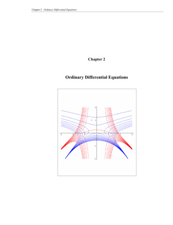
Chapter 2 Ordinary Differential EquationsChapter 2Ordinary Differential Equations
Chapter 2 Ordinary Differential EquationsChapter 2Ordinary Differential Equations2.1 Basic concepts, definitions, notations and classificationIntroduction – modeling in engineeringDifferential equation - DefinitionOrdinary differential equation (ODE)Partial differential equations (PDE)Differential operator DOrder of DELinear operatorLinear and non-linear DEHomogeneous ODENon-homogeneous ODENormal form of nth order ODESolution of DEAnsatzExplicit solution (implicit solution integral)Trivial solutionComplete solutionGeneral solutionParticular solutionIntegral curveInitial Value ProblemBoundary Value ProblemTypes of Boundary Conditions:I) boundary condition of the Ist kind (Dirichlet boundary conditionII) boundary condition of the IInd kind (Neumann boundary condition)III) boundary condition of the IIIrd kind (Robin or mixed boundary condition)Well-posed or ill-posed BVPUniqueness of solutionSingular point2.2 First order ODENormal and Standard differential formsPicard’s Theorem (existence and uniqueness of the solution of IVP)2.2.1Exact ODEExact differentialPotential functionExact differential equationTest on exact differentialSolution of exact equation2.2.2Equations Reducible to Exact - Integrating FactorIntegrating factorSuppressed solutionsReduction to exact equation2.2.3Separable equationsSeparable equationSolution of separable equation
Chapter 2 Ordinary Differential Equations2.2.4Homogeneous EquationsHomogeneous functionHomogeneous equationReduction to separable equation – substitutionHomogeneous functions in R n2.2.5Linear 1st order ODEGeneral solutionSolution of IVP2.2.6 Special EquationsBernoulli EquationRicatti equationClairaut equationLagrange equationEquations solvable for y2.2.7 Applications of first order ODE1.Orthogonal trajectoriesFamily of trajectoriesSlope of tangent lineOrthogonal linesOrthogonal trajectoriesAlgorithm2.2.8 Approximate and Numerical methods for 1st order ODEDirection field – method of isoclinesEuler’s Method, modified Euler methodThe Runge-Kutta MethodPicard’s Method of successive approximationsNewton’s Method (Taylor series solution)Linearization2.2.9 Equations of reducible order1. The unknown function does not appear in an equation explicitly2. The independent variable does not appear in the equation explicitly(autonomous equation)3. Reduction of the order of a linear equation if one solution is known2.3 Theory of Linear ODE2.3.1.Linear ODEInitial Value ProblemExistence and uniqueness of solution of IVP2.3. 2Homogeneous linear ODELinear independent sets of functionsWronskianSolution space of L n y 0Fundamental setComplimentary solution
Chapter 2 Ordinary Differential Equations2.3.3Non-Homogeneous linear ODEGeneral solution of L n y f (x )Superposition principle2.3.4Fundamental set of linear ODE with constant coefficients2.3.5.Particular solution of linear ODEVariation of parameterUndetermined coefficients2.3.6.Euler-Cauchy Equation2.4 Power Series Solutions2.4.1Introduction2.4.2Basic definitions and resultsOrdinary pointsBinomial coefficients etc.Some basic facts on power seriesReal analytic functions2.4.3The power series methodExistence and uniqueness of solutionsAnalyticity of the solutionsDetermining solutions2.5 The Method of Frobenius2.5.1Introduction2.5.2Singular points2.5.3The solution method2.5.4The Bessel functions2.6 Exercises
Chapter 2 Ordinary Differential Equations2.1 Basic concepts, definitions, notations and classificationEngineering design focuses on the use of models in developing predictions ofnatural phenomena. These models are developed by determining relationshipsbetween key parameters of the problem. Usually, it is difficult to findimmediately the functional dependence between needed quantities in the model;at the same time, often, it is easy to establish relationships for the rates ofchange of these quantities using empirical laws. For example, in heat transfer,directional heat flux is proportional to the temperature gradient (Fourier’s Law)dTq kdxwhere the coefficient of proportionality is called the coefficient of conductivity.Also, during light propagation in the absorbing media, the rate of change ofintensity I with distance is proportional to itself (Lambert’s Law)dI kIdswhere the coefficient of proportionality is called the absorptivity of the media.In another example, if we are asked to derive the path x(t ) of a particle of massm moving under a given time-dependent force f (t ) , it is not easy to find itdirectly, however, Newton’s second law (acceleration is proportional to theforce) gives a differential equation describing this motion.d 2 x(t )m f (t )dt 2The solution of which gives an opportunity to establish the dependence of pathon the acting force.The basic approach to deriving models is to apply conservation laws andempirical relations for control volumes. In most cases, the governing equationfor a physical model can be derived in the form of a differential equation. Thegoverning equations with one independent variable are called ordinarydifferential equations. Because of this, we will study the methods of solution ofdifferential equations.Differential equationDefinition 1Example 1:A differential equation is an equation, which includes at leastone derivative of an unknown function.dy (x ) 2 xy (x ) e xdx2b) y ( y ′′) y ′ sin xa)c) 2 u ( x, y ) 2 u ( x, y ) 0 y 2 x 2()d) F x , y , y′,., y (n ) 0e) 2u (x ,t ) u (x , t ) v 0 x x 2If a differential equation (DE) only contains unknown functions of one variableand, consequently, only the ordinary derivatives of unknown functions, then thisequation is said to be an ordinary differential equation (ODE); in a case whereother variables are included in the differential equation, but not the derivativeswith respect to these variables, the equation can again be treated as an ordinarydifferential equation in which other variables are considered to be parameters.Equations with partial derivatives are called partial differential equations
Chapter 2 Ordinary Differential Equations(PDE). In Example 1, equations a),b) and d) are ODE’s, and equation c) is aPDE; equation e) can be considered an ordinary differential equation with theparameter t .Differential operator DOrder of DELinear operatorIt is often convenient to use a special notation when dealing with differentialequations. This notation called differential operators, transformsfunctions into the associated derivatives. Consecutive application of theoperator D transforms a differentiable function f (x ) into its derivatives ofdifferent orders:df (x )Df (x ) D: f f ′dxd 2 f (x )D 2 f (x ) D 2 : f f ′′2dxA single operator notation D can be used for application of combinations ofoperators; for example, the operatorD aD n bDimpliesd n f (x )df (x )Df (x ) aD n f (x ) bDf (x ) a bndxdxThe order of DE is the order of the highest derivative in the DE. It can bereflected as an index in the notation of the differential operator asD 2 aD 2 bD cThen a differential equation of second order with this operator can be written inthe compact formD 2 y F (x )A differential operator D n is linear if its application to a linear combination ofn times differentiable functions f (x ) and g (x ) yields a linear combinationD n (αf βg ) αD n f βD n g , α , β RThe most general form of a linear operator of nth order may be written asL n a 0 (x )D n a1 (x )D n 1 a n 1 (x )D a n (x )where the coefficients ai ( x ) C ( R ) are continuous functions.Linear and non-linear DEA DE is said to be linear, if the differential operator defining this equation islinear. This occurs when unknown functions and their derivatives appear asDE’s of the first degree and not as products of functions combinations of otherfunctions. A linear DE does not include terms, for example, like the following:3y 2 , ( y ′) , yy ′ , ln ( y ) , etc.If they do, they are referred to as non-linear DE’s.A linear ODE of the nth order has the formL n y (x ) a 0 (x ) y (n ) (x ) a1 (x ) y (n 1) (x ) a n 1 (x ) y ′(x ) a n (x ) y (x ) F (x )where the coefficients a i (x ) and function F (x ) are, usually, continuousfunctions. The most general form of an nth order non-linear ODE can beformally written asF x, y, y ′,., y (n ) 0which does not necessarily explicitly include the variable x and unknownfunction y with all its derivatives of order less than n.()A homogeneous linear ODE includes only terms with unknown functions:L n y (x ) 0A non-homogeneous linear ODE involves a free term (in general, a function ofan independent variable):
Chapter 2 Ordinary Differential EquationsLn y (x ) F (x )A normal form of an nth order ODE is written explicitly for the nth derivative:y (n ) f x, y, y ′,., y (n 1)(Solution of DEDefinition 2)Any n times differentiable function y (x ) which satisfies a DE()F x, y, y ′,., y (n ) 0is called a solution of the DE, i.e. substitution of functiony (x ) into the DE yields an identity.“Satisfies” means that substitution of the solution into the equation turns it intoan identity. This definition is constructive – we can use it as a trial method forfinding a solution (guess a form of a solution (which in modern mathematics isoften called ansatz), substitute it into the equation and force the equation to bean identity).Example 2:Consider the ODE y ′ y 0 on x I ( , )Look for a solution in the form y e axSubstitution into the equation yieldsae ax e ax 0(a 1)e ax 0 divide by e ax 0a 1 0 a 1Therefore, the solution is y e x .But this solution is not necessarily a unique solution of theODE.The Solution of the ODE may be given by an explicit expression like in example2 called the explicit solution; or by an implicit function (called the implicitsolution integral of the differential equation)g ( x, y ) 0If the solution is given by a zero function y (x ) 0 , then it is called to be atrivial solution. Note, that the ODE in example 2 posses also a trivial solution.The complete solution of a DE is a set of all its solutions.The general solution of an ODE is a solution which includes parameters, andvariation of these parameters yields a complete solution.Thus, y ce x , c R is a complete solution of the ODE in example 2.The general solution of an nth order ODE includes n independent parameters andsymbolically can be written asg (x, y, c1 ,., c n ) 0The particular solution is any individual solution of the ODE. It can beobtained from a general solution with particular values of parameters. Forexample, e x is a particular solution of the ODE in example 2 with c 1 .{}A solution curve is a graph of an explicit particular solution. An integralcurve is defined by an implicit particular solution.The differential equationyy ′ 1has a general solutiony2 x c2The integral curves are implicit graphs of the general solution for differentvalues of the parameter cExample 3:
Chapter 2 Ordinary Differential EquationsTo get a particular solution which describes the specified engineering model, theinitial or boundary conditions for the differential equation should be set.Initial Value ProblemAn initial value problem (IVP) is a requirement to find a solution of nth orderODEF x, y, y ′,., y (n ) 0 for x I subject to n conditions on the solution y (x ) and its derivatives up to order n-1specified at one point x 0 I :y (x 0 ) y 0y ′(x 0 ) y1()y (n 1) (x 0 ) y n 1where y0 , y1 ,., yn 1 Boundary Value Problem.In a boundary value problem (BVP), the values of the unknown function and/orits derivatives are specified at the boundaries of the domain (end points of theinterval (possibly )).For example,find the solution of y ′′ y x 2 on x [a, b]satisfying boundary conditions:y (a ) yay (b ) ybwhere ya , yb The solution of IVP’s or BVP’s consists of determining parameters in thegeneral solution of a DE for which the particular solution satisfies specifiedinitial or boundary conditions.Types of Boundary ConditionsI) a boundary condition of the Ist kind (Dirichlet boundary condition) specifiesthe value of the unknown function at the boundary x L :u x L fII) a boundary condition of the IInd kind (Neumann boundary condition)specifies the value of the derivative of the unknown function at the boundaryx L (flux):du fdx x LIII) a boundary condition of the IIIrd kind (Robin boundary condition or mixedboundary condition) specifies the value of the combination of the unknownfunction with its derivative at the boundary x L (a convective type boundarycondition) du f k dx hu x L
Chapter 2 Ordinary Differential EquationsBoundary value problems can be well-posed or ill-posed.Uniqueness of solutionThe solution of an ODE is unique at the point (x 0 , y 0 ) , if for all values ofparameters in the general solution, there is only one integral curve which goesthrough this point. Such a point where the solution is not unique or does notexist is called a singular point.The question of the existence and uniqueness of the solution of an ODE is veryimportant for mathematical modeling in engineering. In some cases, it ispossible to give a general answer to this question (as in the case of the first orderODE in the next section.)Example 4:a) The general solution of the ODE in Example 2 is{ y ce x},c RThere exists a unique solution at any point in the planeb) Consider the ODE xy ′ 2 y 0{}The general solution of this equation is y cx 2 ,c R(0,0) is a singular point for this ODE
Chapter 2 Ordinary Differential Equations2.2 First order ODEnormal formstandard differential formIn this section we will consider the first order ODE, the general form of whichis given byF ( x, y , y ′ ) 0This equation may be linear or non-linear, but we restrict ourselves mostly toequations which can be written in normal form (solved with respect to thederivative of the unknown function):y ′ f ( x, y )or in the standard differential form:M (x, y )dx N (x, y )dy 0Note that the equation in standard form can be easily transformed to normalform and vice versa. If the equation initially was given in general form, thenduring transformation to normal or standard form operations (like division orroot extraction) can eliminate some solutions, which are called suppressedsolutions. Therefore, later we need to check for suppressed solutions.Initial Value ProblemIn an initial value problem (IVP) for a first order ODE, it is required to find asolution ofF (x, y, y ′) 0 for x I Rsubject to the initial condition at x 0 I :y (x 0 ) y 0 , y0 RBoundary value problems will differ only by fixing x0 at the boundary of theregion I.The question of existence and uniqueness of the solution of an IVP for the firstorder ODE can be given in the form of sufficient conditions for equations innormal form by Picard’s Theorem:Picard’s TheoremTheorem (existence and uniqueness of the solution of IVP)Let the domain R be a closed rectangle centered at the point( x0 , y 0 ) R 2 :R {( x, y ) R2}: x x0 a, y y0 band let the function f (x, y ) be continuous and continuouslydifferentiable in terms of the y function in the domain R:f (x, y ) C [R ]f y (x, y ) C [R ]and let the function f (x, y ) be bounded in R:f (x, y ) M for (x, y ) R .Then the initial value problemy ′ f ( x, y )y ( x0 ) y 0has a unique solution y ( x ) in the interval b I {x : x x0 h}, where h min a, M The proof of Picard’s theorem will be given in the following chapters; it also canbe found in Hartmann [ ], Perco [ ] etc. and it is based on Picard’s successfulapproximations to the solution of IVP which we will consider later. Thistheorem guarantees that under given conditions there exists a unique solution ofthe IVP, but it does not claim that the solution does not exist if conditions of thetheorem are violated. Now we will consider the most important methods ofsolution of the first order ODE
Chapter 2 Ordinary Differential Equations
Chapter 2 Ordinary Differential Equations2.2.1 Exact ODEConsider a first order ODE written in the standard differential form:M (x, y )dx N (x, y )dy 0 ,( x, y ) D 2exact differential(1)If there exists a differentiable function f (x, y ) such that f (x, y ) M ( x, y )(2) x f (x, y ) N ( x, y )(3) yfor all (x, y ) D , then the left hand side of the equation is an exact differentialof this function, namely f fdf dx dy M (x, y )dx N (x, y )dy x yand the function f (x, y ) satisfying conditions (2) and (3) is said to be apotential function for equation (1). The equation in this case is called to be anexact differential equation, which can be written asdf (x, y ) 0(4)direct integration of which yields a general solution of equation (1):f ( x, y ) c(5)where c R is a constant of integration. The solution given implicitly definesintegral curves of the ODE or the level curves of function f (x, y ) .Example 1The First order ODE 3x 2 dx 2 ydy 0 is an exact equationwith the general solutionf ( x, y ) x 3 y 2 c . Then theintegral curves of this equation areTo recognize that a differential equation is an exact equation we can use a testgiven by the following theorem:Test on exact differentialTheorem 1 (Euler, 1739)Let functions M (x, y ) and N (x, y ) be continuouslydifferentiable on D 2 , then the differential formM (x, y )dx N (x, y )dyis an exact differential if and only if M N y xin D 2(6)(7)Proof: 1) Suppose that the differential form is exact. According to definition, it f (x, y )means that there exists a function f (x, y ) such that M (x, y ) and x f (x, y ) N (x, y ) . Then differentiating the first of these equations with respect y
Chapter 2 Ordinary Differential Equationsto y and the second one with respect to x, we get 2 f (x, y ) M (x, y ) and x y y 2 f (x, y ) N (x, y ) . Since the left hand sides of these equations are the same, x y x M Nit follows that . y x M N2) Suppose now that the condition holds for all (x, y ) D . y xTo show that there exists a function f (x, y ) which produces an exact differentialof the form (6), we will construct such a function. The same approach is usedfor finding a solution of an exact equation.We are looking for a function f (x, y ) , the differential form (6) of which isan exact differential. Then this function should satisfy conditions (2) and (3).Take the first of these conditions: f (x, y ) M ( x, y ) xand integrate it formally over variable x, treating y as a constant, thenf (x, y ) M (x, y )dx k ( y )(8)where the constant of integration depends on y. Differentiate this equation withrespect to y and set it equal to condition (3): f (x, y ) dk ( y ) N ( x, y )M (x, y )dx dy y yRearrange the equation as shown dk ( y ) N ( x, y ) M (x, y )dx y dyThen integration over the variable y yields: k ( y ) N ( x, y ) M (x, y )dx dy c1 y Substitute this result into equation (8) instead of k ( y ) f (x, y ) M (x, y )dx N (x, y ) M (x, y )dx dy c1(9) y To show that this function satisfies conditions (2) and (3), differentiate it withrespect to x and y and use condition (7). Therefore, differential form (6) is anexact differential of the function f (x, y ) constructed in equation (9).The other form of the function f (x, y ) can be obtained if we start first withcondition (3) instead of condition (2): f (x , y ) N (x , y )dy M (x , y ) N (x , y )dx dx c 2(10) x Note, that condition (7) was not used for construction of functions (9) or (10),we applied it only to show that form (6) is an exact differential of these functions.Then according to equation (5), a general solution of exact equation is given byan implicit equations:or f ( x, y ) M ( x, y ) dx N ( x, y ) M ( x, y ) dx dy c y (11) f ( x, y ) N ( x, y ) dy M ( x, y ) N ( x, y ) dx dx c x (12)
Chapter 2 Ordinary Differential EquationsThe other form of the general solution can be obtained by constructing afunction with help of a definite integration involving an arbitrary point (x0 , y0 )in the region D 2:xyx0y0f (x, y ) M (t , y )dt N (x0 , t )dt cxyx0y0f (x, y ) M (t , y0 )dt N (x, t )dt c(13)(14)Formulas (1) and (12) or (13) and (14) are equivalent – they should produce thesame solution set of differential equation (1), but actual integration may be moreconvenient for one of them.Example 2 Find a complete solution of the following equation(3 y x )dx ( y 3x )dy 0Test for exactness: N M 3 3 the equation is exact x yWe can apply eqns. 11-14, but in practice, usually, it is more convenient to usethe same steps to find the function f ( x, y ) as in the derivation of the solution.Start with one of the conditions for the exact differential f (x, y ) M ( x, y ) ( 3 y x ) xIntegrate it over x , treating y as a parameter (this produces a constant ofintegration k ( y ) depending on y )x2 k ( y)2Use the second condition for the exact differential f ( x, y ) N ( x, y ) 3x y yf ( x, y ) 3 yx 3x k ( y ) y k ( y ) y 3x y ySolve this equation for k ( y )y22neglecting the constant of integration. The function is completely determinedand the solution of the ODE is given byx2 y 2f ( x, y ) 3 yx c22or we can rewrite it as a general solution given by the implicit equation:k ( y) General solution:x 2 6 xy y 2 0Solution curves:
Chapter 2 Ordinary Differential EquationsNote that at the point (0,0) the solution is not unique.Where also conditions of Picard’s theorem are violated?The solution with help from equation 13:Choose x0 0 , y0 0 , thenyxf ( x, y ) ( 3 y t ) dt ( 0 t ) dt c0x0y t t 3 yt c2 0 2 0 22x2 y2 c22This is the same solution as in the first approach.3 yx 2.2.2Equations Reducible to Exact - Integrating FactorIntegrating factorIn general, non-exact equations, which possess a solution, can be transformed toexact equations after multiplication by some nonzero function µ (x, y ) , which iscalled an integrating factor (existence of the integral factor was proved byEuler).Theorem 2The function µ (x , y ) is an integrating factor of the differentialequation M (x, y )dx N (x, y )dy 0 if and only if µ (x , y )satisfies the partial differential equation µ N M µ µ M N x x y y Proof: as an exerciseBut it is not always easy to find this integrating factor. There are several specialcases for which the integrating factor can be determined:1) M N 0 y x M N y x2) f (x )NThe test for exactness. The integrating factorµ (x , y ) 1The test for exactness fails but the givenratio is a function of x only. Then theintegrating factor isµ (x ) e f ( x )dx
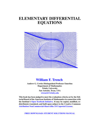
Chapter 2 Ordinary Differential Equations 3) M N y x g(y)MThe test for exactness fails but the givenratio is a function of y only. Then theintegrating factor isµ ( y ) e M N y x4) h(xy )yN xMg ( y ) dyThe test for exactness fails but the givenratio is a function of the product of x andy . Then the integrating factor isµ (x , y ) h(xy )d (xy ) M N y 2 x y y5) k xM yN x The test for exactness fails but the givenratio is a function of the ratiox. Then theyintegrating factor is y y x x µ (x , y ) k d 6)M (λx , λy ) M (x , y ) N (λx , λy ) N (x , y )The functions M and N are homogeneousfunctions of the same degree (see section).Then the integrating factor is1µ (x , y ) xM yNproviding xM yN 0 .Example 3 Find a complete solution of the following equationx y 2 dx 2 xydy 0Test for exactness: M N 2y equation is not exact 2 y y x()test for integrating factor: M N 2 y ( 2 y ) 2 y x f (x )Nx 2 xyµ (x ) e f ( x )dx e 2 int.factor by Eq. 211 x dx e 2 ln x e ln x 122x(x y ) dx 2 y dy 02x2xx y f1 y2 x x2 xx22 f ln x y2 kx f2 y k 2 y k c yx yx
Chapter 2 Ordinary Differential EquationsGeneral solution:y2 ln x cx cx e(Is x 0 a suppressed solution: x y 2y2xdx) dy 2 xy 0(yes)Illustration of this problem with Maple: restart; with(plots): f: {seq(log(abs(x))-y 2/x i,i -10.10)}: implicitplot(f,x 1.1,y 2.2,numpoints 6000);Solution with Maple: restart; with(DEtools): DE: diff(y(t),t)*2*y(t)*t y(t) 2 t; DE : 2 y( t ) y( t ) t y( t ) 2 t t s: dsolve(DE,y(t));s : y( t ) t ln( t ) t C1 , y( t ) t ln( t ) t C1 restart; q: {seq(y(t) 2 t*ln(abs(t)) t*i/4,i -8.8)}: with(plots): implicitplot(q,t -10.10,y 2.2,numpoints 5000);
Chapter 2 Ordinary Differential EquationsSupressed solutionsIf the given differential equation is reduced to standard differential formM (x, y )dx N (x, y )dy 0with some algebraic operations, then zeros of the expressions involved indivision can be solutions of the differential equation not included in the generalsolution. Such lost solutions are called suppressed solutions. If suchoperations were applied for the transformation of the differential equation, thenthe equation has to be checked for suppressed solutions.To check if y a is a suppressed solution of Eq. 1, reduce the differentialequation to normal form with y as a dependent variabledy M (x , y ) dxN (x , y )and substitute y a .To check if x b is a suppressed solution of Eq. 1, reduce the differentialequation to normal form with x as a dependent variabledx N (x , y ) dy M (x , y )and substitute x b .Then the suppressed solutions should be added to the general solution.
Chapter 2 Ordinary Differential EquationsSolid Geometry
Chapter 2 Ordinary Differential Equations2.2.3 Separable equationsSeparable equationDefinition 1A differential equation of the first order is called separable ifit can be written in the following standard differential form:M 1 (x )M 2 ( y )dx N 1 (x )N 2 ( y )dy 0where(1)M 1 (x ), N 1 (x ) are functions of the variable x only andM 2 ( y ), N 2 ( y ) are functions of the variable y only.Assuming that N 1 (x ) 0 and M 2 ( y ) 0 for all x and y in the range, variablesin equation (1) can be separated by division with M 2 ( y )N 1 (x ) :N (y)M 1 (x )dy 0dx 2M 2 (y)N 1 (x )Then equation (2) can be formally integrated to obtain a general solution: M 1 (x )N (y)dx 2dy cN 1 (x )M 2 (y)(2)(3)where c R is an arbitrary constant.Note, that separated equation (2) is exact - it can be obtained from equation (1)1; the potentialby multiplication by the integrating factor µ N 1 (x )M 2 ( y )function for this equationN (y)M (x )dyf (x, y ) 1 dx 2M 2 (y)N 1 (x )Which yields the same general solution f (x, y ) c .Because of division by M 2 ( y )N 1 (x ) , some solutions can be lost; therefore,equations should be checked for suppressed solutions. If x x1 , where x1 Rbelongs to the domain and is a root of N 1 (x ) 0 , then the function x x1 isobviously a solution of differential equation (1). Similarly, if y y1 is a realroot of M 2 ( y ) 0 , then the function y y1 is also a solution. They bothshould be added to the general solution (3).Example 1: Find a general solution of the following ODE:xyy ′ y 2 1 ln x 0 ,x 0( )xydy (y 1) ln xdx 02yln xdx 2dy 0xy 1(ln x )2 ln(y 2 1) cno suppressed solutions
Chapter 2 Ordinary Differential EquationsExample 6Find a solution of the following ODE:(xSolution:2) 4 y ′ x cot y 0Separate variables:xdx tan ydy 0x2 4Integrate:ln ( cos y ) ln x 2 4 ln c2General solution:(x2) 4 cos 2 y cCheck for suppressed solutions:y π2 nπ are suppressed solutions.()dx 0dyif independent and dependent variables are reversed.x 2 are solutions of x 2 4 (x tan y )Then the family of solution curves is represented byy y 3π2π2y y π23π2
Chapter 2 Ordinary Differential Equations2.2.4 Homogeneous EquationsIn this section, we will study a type of equations which can be reduced to aseparable equation or to an exact equation.Homogeneous functionDefinition 1 Function M (x, y ) is homogeneous of degree r, ifM (λx, λy ) λ r M (x, y ) for any λ R , λ 0It means that after replacing x by λx and y by λy in the function M (x, y ) ,the parameter λ r can be factored from the expression.Examples 1:a) Homogeneous function of degree zero.x y, thenLetM ( x, y ) x yM (λx, λy ) λx λy x y λ 0 M ( x, y ) M ( x , y )λx λy x yfor λ 0Therefore, M (x, y ) is homogeneous of degree zero.If we divide the numerator and the denominator by x, theny1 xM (x , y ) y1 xand we see that the function M (x , y ) depends on a single variabley.xIt appears to be a fact for zero degree homogeneous functions:the function M (x , y ) is homogeneous of degree zero if and only if it dependsy[Goode, p.62]:x y M (x , y ) f x on a single variableb) A more general fact: homogeneous functions of degree r can be written as y x n M ( x, y ) f or x x y n M ( x, y ) g y 1 To show it, choose parameters of the form λ x 1 xc) Consider M (x , y ) M (λx , λy ) x 0x 0y 3 x 2 y . Test on homogeneity yields(λy )3 (λx )2 λy λ 2 3y 3 x 2 y λ 2 3 M (x , y )Therefore, the given function is homogeneous of degree 3 2 .
Chapter 2 Ordinary Differential EquationsA Differential equation written in standard differential formM (x , y )dx N (x , y )dy 0is called a homogeneous differential equation if functionsM (x, y ) and N (x , y ) are homogeneous of the same degree r.Homogeneous equationDefinition 2Reduction to separableIf the equation written in standard differential formM (x , y )dx N (x , y )dy 0is homogeneous, then it can be reduced to a separable differential equation bythe change of variable:y uxdy xdu udxorx vydx vdy ydvBoth approaches are equivalent, just because in standard differential form thevariables are equivalent. But actual integration of the equation may be moreconvenient with one of them.Justification: First apply the substitution to the differential equation y
Chapter 2 Ordinary Differential Equations (PDE). In Example 1, equations a),b) and d) are ODE's, and equation c) is a PDE; equation e) can be considered an ordinary differential equation with the parameter t. Differential operator D It is often convenient to use a special notation when dealing with differential equations.