Transcription
1INTRODUCTION TO DIFFERENTIALEQUATIONS1.1 Definitions and Terminology1.2 Initial-Value Problems1.3 Differential Equations as Mathematical ModelsCHAPTER 1 IN REVIEWThe words differential and equations certainly suggest solving some kind ofequation that contains derivatives y , y , . . . . Analogous to a course in algebra andtrigonometry, in which a good amount of time is spent solving equations such asx2 5x 4 0 for the unknown number x, in this course one of our tasks will beto solve differential equations such as y 2y y 0 for an unknown functiony (x).The preceding paragraph tells something, but not the complete story, about thecourse you are about to begin. As the course unfolds, you will see that there is moreto the study of differential equations than just mastering methods that someone hasdevised to solve them.But first things first. In order to read, study, and be conversant in a specializedsubject, you have to learn the terminology of that discipline. This is the thrust of thefirst two sections of this chapter. In the last section we briefly examine the linkbetween differential equations and the real world. Practical questions such as Howfast does a disease spread? How fast does a population change? involve rates ofchange or derivatives. As so the mathematical description—or mathematicalmodel —of experiments, observations, or theories may be a differential equation.1
2 CHAPTER 11.1INTRODUCTION TO DIFFERENTIAL EQUATIONSDEFINITIONS AND TERMINOLOGYREVIEW MATERIAL Definition of the derivativeRules of differentiationDerivative as a rate of changeFirst derivative and increasing/decreasingSecond derivative and concavityINTRODUCTION The derivative dy dx of a function y (x) is itself another function (x)2found by an appropriate rule. The function y e0.1x is differentiable on the interval ( , ), and20.1x 2by the Chain Rule its derivative is dy dx 0.2xe . If we replace e0.1x on the right-hand side ofthe last equation by the symbol y, the derivative becomesdy 0.2xy.dx(1)Now imagine that a friend of yours simply hands you equation (1) —you have no idea how it wasconstructed —and asks, What is the function represented by the symbol y? You are now face to facewith one of the basic problems in this course:How do you solve such an equation for the unknown function y (x)?A DEFINITION The equation that we made up in (1) is called a differentialequation. Before proceeding any further, let us consider a more precise definition ofthis concept.DEFINITION 1.1.1 Differential EquationAn equation containing the derivatives of one or more dependent variables,with respect to one or more independent variables, is said to be a differentialequation (DE).To talk about them, we shall classify differential equations by type, order, andlinearity.CLASSIFICATION BY TYPE If an equation contains only ordinary derivatives ofone or more dependent variables with respect to a single independent variable it issaid to be an ordinary differential equation (ODE). For example,A DE can contain morethan one dependent variablebdy 5y ex,dx2d y dy 6y 0,dx2 dxandbdx dy 2x ydtdt(2)are ordinary differential equations. An equation involving partial derivatives ofone or more dependent variables of two or more independent variables is called a
1.1DEFINITIONS AND TERMINOLOGY 3partial differential equation (PDE). For example,22uu 0,2xy222uuu 2 ,22xttanduv yx(3)are partial differential equations.*Throughout this text ordinary derivatives will be written by using either theLeibniz notation dy dx, d 2 y dx 2, d 3 y dx 3, . . . or the prime notation y , y , y , . . . .By using the latter notation, the first two differential equations in (2) can be writtena little more compactly as y 5y e x and y y 6y 0. Actually, the primenotation is used to denote only the first three derivatives; the fourth derivative iswritten y (4) instead of y . In general, the nth derivative of y is written d n y dx n or y (n).Although less convenient to write and to typeset, the Leibniz notation has an advantage over the prime notation in that it clearly displays both the dependent andindependent variables. For example, in the equationunknown functionor dependent variabled 2x––– 16x 0dt 2independent variableit is immediately seen that the symbol x now represents a dependent variable,whereas the independent variable is t. You should also be aware that in physicalsciences and engineering, Newton’s dot notation (derogatively referred to by someas the “flyspeck” notation) is sometimes used to denote derivatives with respectto time t. Thus the differential equation d 2s dt 2 32 becomes s̈ 32. Partialderivatives are often denoted by a subscript notation indicating the independent variables. For example, with the subscript notation the second equation in(3) becomes u xx u tt 2u t.CLASSIFICATION BY ORDER The order of a differential equation (eitherODE or PDE) is the order of the highest derivative in the equation. For example,second orderfirst order( )dy 3d 2y––––2 5 ––– 4y e xdxdxis a second-order ordinary differential equation. First-order ordinary differentialequations are occasionally written in differential form M(x, y) dx N(x, y) dy 0.For example, if we assume that y denotes the dependent variable in(y x) dx 4x dy 0, then y dy dx, so by dividing by the differential dx, weget the alternative form 4xy y x. See the Remarks at the end of this section.In symbols we can express an nth-order ordinary differential equation in onedependent variable by the general formF(x, y, y , . . . , y(n)) 0,(4)where F is a real-valued function of n 2 variables: x, y, y , . . . , y (n). For both practical and theoretical reasons we shall also make the assumption hereafter that it ispossible to solve an ordinary differential equation in the form (4) uniquely for the*Except for this introductory section, only ordinary differential equations are considered in A FirstCourse in Differential Equations with Modeling Applications, Ninth Edition. In that text theword equation and the abbreviation DE refer only to ODEs. Partial differential equations or PDEsare considered in the expanded volume Differential Equations with Boundary-Value Problems,Seventh Edition.
4 CHAPTER 1INTRODUCTION TO DIFFERENTIAL EQUATIONShighest derivative y (n) in terms of the remaining n 1 variables. The differentialequationd ny f (x, y, y , . . . , y(n 1)),dxn(5)where f is a real-valued continuous function, is referred to as the normal form of (4).Thus when it suits our purposes, we shall use the normal formsdy f (x, y)dxd 2y f (x, y, y )dx2andto represent general first- and second-order ordinary differential equations. For example,the normal form of the first-order equation 4xy y x is y (x y) 4x; the normalform of the second-order equation y y 6y 0 is y y 6y. See the Remarks.CLASSIFICATION BY LINEARITY An nth-order ordinary differential equation (4)is said to be linear if F is linear in y, y , . . . , y (n). This means that an nth-order ODE islinear when (4) is a n(x)y (n) a n 1(x)y (n 1) a1(x)y a 0 (x)y g(x) 0 oran(x)dnyd n 1y a(x) n 1dx ndx n 1 a1(x)dy a0(x)y g(x).dx(6)Two important special cases of (6) are linear first-order (n 1) and linear secondorder (n 2) DEs:a1(x)dy a0 (x)y g(x)dxanda2 (x)d 2ydy a1(x) a0 (x)y g(x). (7)dx2dxIn the additive combination on the left-hand side of equation (6) we see that the characteristic two properties of a linear ODE are as follows: The dependent variable y and all its derivatives y , y , . . . , y (n) are of thefirst degree, that is, the power of each term involving y is 1. The coefficients a 0, a1, . . . , a n of y, y , . . . , y (n) depend at most on theindependent variable x.The equations(y x)dx 4x dy 0,y 2y y 0,andd 3ydy x 5y exdx3dxare, in turn, linear first-, second-, and third-order ordinary differential equations. Wehave just demonstrated that the first equation is linear in the variable y by writing it inthe alternative form 4xy y x. A nonlinear ordinary differential equation is simply one that is not linear. Nonlinear functions of the dependent variable or its derivatives, such as sin y or e y , cannot appear in a linear equation. Thereforenonlinear term:coefficient depends on ynonlinear term:nonlinear function of y(1 y)y 2y ex,d 2y––––2 sin y 0,dxnonlinear term:power not 1andd 4y––––4 y 2 0dxare examples of nonlinear first-, second-, and fourth-order ordinary differential equations, respectively.SOLUTIONS As was stated before, one of the goals in this course is to solve, orfind solutions of, differential equations. In the next definition we consider the concept of a solution of an ordinary differential equation.
1.1DEFINITIONS AND TERMINOLOGY 5DEFINITION 1.1.2 Solution of an ODEAny function , defined on an interval I and possessing at least n derivativesthat are continuous on I, which when substituted into an nth-order ordinarydifferential equation reduces the equation to an identity, is said to be asolution of the equation on the interval.In other words, a solution of an nth-order ordinary differential equation (4) is a function that possesses at least n derivatives and for whichF(x, (x), (x), . . . , (n)(x)) 0for all x in I.We say that satisfies the differential equation on I. For our purposes we shall alsoassume that a solution is a real-valued function. In our introductory discussion we2saw that y e0.1x is a solution of dy兾dx 0.2xy on the interval ( , ).Occasionally, it will be convenient to denote a solution by the alternativesymbol y(x).INTERVAL OF DEFINITION You cannot think solution of an ordinary differentialequation without simultaneously thinking interval. The interval I in Definition 1.1.2is variously called the interval of definition, the interval of existence, the intervalof validity, or the domain of the solution and can be an open interval (a, b), a closedinterval [a, b], an infinite interval (a, ), and so on.EXAMPLE 1Verification of a SolutionVerify that the indicated function is a solution of the given differential equation onthe interval ( , ).1(a) dy dx xy1/2; y 16 x4(b) y 2y y 0; y xexSOLUTION One way of verifying that the given function is a solution is to see, aftersubstituting, whether each side of the equation is the same for every x in the interval.(a) Fromleft-hand side:11dy (4 x3) x3,dx 164right-hand side:xy1/2 x 1 4x161/2 x 14 x 14 x ,23we see that each side of the equation is the same for every real number x. Note11that y1/2 4 x2 is, by definition, the nonnegative square root of 16 x4 .(b) From the derivatives y xe x e x and y xe x 2e x we have, for every realnumber x,left-hand side:y 2y y (xex 2ex ) 2(xex ex ) xex 0,right-hand side:0.Note, too, that in Example 1 each differential equation possesses the constant solution y 0, x . A solution of a differential equation that is identicallyzero on an interval I is said to be a trivial solution.SOLUTION CURVE The graph of a solution of an ODE is called a solutioncurve. Since is a differentiable function, it is continuous on its interval I of definition. Thus there may be a difference between the graph of the function and the
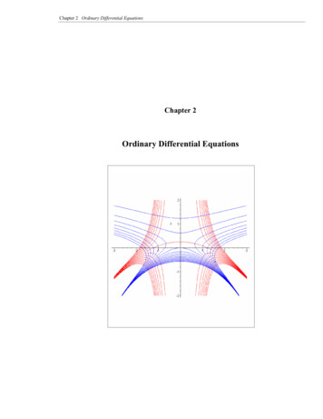
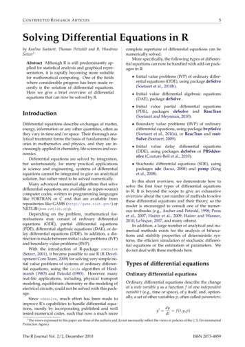
6 CHAPTER 1INTRODUCTION TO DIFFERENTIAL EQUATIONSgraph of the solution . Put another way, the domain of the function need not bethe same as the interval I of definition (or domain) of the solution . Example 2illustrates the difference.yEXAMPLE 211x(a) function y 1/x, x 苷 0yFunction versus SolutionThe domain of y 1 x, considered simply as a function, is the set of all real numbers x except 0. When we graph y 1 x, we plot points in the xy-plane corresponding to a judicious sampling of numbers taken from its domain. The rationalfunction y 1 x is discontinuous at 0, and its graph, in a neighborhood of the origin, is given in Figure 1.1.1(a). The function y 1 x is not differentiable at x 0,since the y-axis (whose equation is x 0) is a vertical asymptote of the graph.Now y 1 x is also a solution of the linear first-order differential equationxy y 0. (Verify.) But when we say that y 1 x is a solution of this DE, wemean that it is a function defined on an interval I on which it is differentiable andsatisfies the equation. In other words, y 1 x is a solution of the DE on any interval that does not contain 0, such as ( 3, 1), 12, 10 , ( , 0), or (0, ). Becausethe solution curves defined by y 1 x for 3 x 1 and 12 x 10 are simply segments, or pieces, of the solution curves defined by y 1 x for x 0and 0 x , respectively, it makes sense to take the interval I to be as large aspossible. Thus we take I to be either ( , 0) or (0, ). The solution curve on (0, )is shown in Figure 1.1.1(b).(11x(b) solution y 1/x, (0, 앝)FIGURE 1.1.1 The function y 1 xis not the same as the solution y 1 x)EXPLICIT AND IMPLICIT SOLUTIONS You should be familiar with the termsexplicit functions and implicit functions from your study of calculus. A solution inwhich the dependent variable is expressed solely in terms of the independentvariable and constants is said to be an explicit solution. For our purposes, let usthink of an explicit solution as an explicit formula y (x) that we can manipulate,evaluate, and differentiate using the standard rules. We have just seen in the last twoexamples that y 161 x4, y xe x, and y 1 x are, in turn, explicit solutionsof dy dx xy 1/2, y 2y y 0, and xy y 0. Moreover, the trivial solution y 0 is an explicit solution of all three equations. When we get down tothe business of actually solving some ordinary differential equations, you willsee that methods of solution do not always lead directly to an explicit solutiony (x). This is particularly true when we attempt to solve nonlinear first-orderdifferential equations. Often we have to be content with a relation or expressionG(x, y) 0 that defines a solution implicitly.DEFINITION 1.1.3 Implicit Solution of an ODEA relation G(x, y) 0 is said to be an implicit solution of an ordinarydifferential equation (4) on an interval I, provided that there exists at leastone function that satisfies the relation as well as the differential equationon I.It is beyond the scope of this course to investigate the conditions under which arelation G(x, y) 0 defines a differentiable function . So we shall assume that ifthe formal implementation of a method of solution leads to a relation G(x, y) 0,then there exists at least one function that satisfies both the relation (that is,G(x, (x)) 0) and the differential equation on an interval I. If the implicit solutionG(x, y) 0 is fairly simple, we may be able to solve for y in terms of x and obtainone or more explicit solutions. See the Remarks.
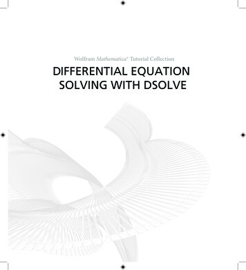
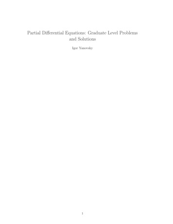
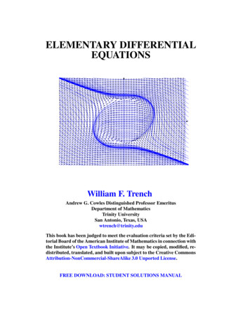
1.1y5DEFINITIONS AND TERMINOLOGY 7EXAMPLE 3 Verification of an Implicit SolutionThe relation x 2 y 2 25 is an implicit solution of the differential equation5xxdy dxy(8)on the open interval ( 5, 5). By implicit differentiation we obtain(a) implicit solutiond 2dd 2x y 25dxdxdxx 2 y 2 25y5xy1 25 x 2, 5 x 5y55x 5(c) explicit solutiony2 25 x 2, 5 x 5FIGURE 1.1.2 An implicit solutionand two explicit solutions of y x yyc 0c 0FIGURE 1.1.3Some solutions ofdy 0.dxAny relation of the form x 2 y 2 c 0 formally satisfies (8) for any constant c.However, it is understood that the relation should always make sense in the real numbersystem; thus, for example, if c 25, we cannot say that x 2 y 2 25 0 is animplicit solution of the equation. (Why not?)Because the distinction between an explicit solution and an implicit solutionshould be intuitively clear, we will not belabor the issue by always saying, “Here isan explicit (implicit) solution.”(b) explicit solutionxy y x 2 sin x2x 2ySolving the last equation for the symbol dy dx gives (8). Moreover, solvingx 2 y 2 25 for y in terms of x yields y 225 x2. The two functionsy 1(x) 125 x2 and y 2(x) 125 x2 satisfy the relation (that is,x 2 12 25 and x 2 22 25) and are explicit solutions defined on the interval( 5, 5). The solution curves given in Figures 1.1.2(b) and 1.1.2(c) are segments ofthe graph of the implicit solution in Figure 1.1.2(a).5c 0orxFAMILIES OF SOLUTIONS The study of differential equations is similar to that ofintegral calculus. In some texts a solution is sometimes referred to as an integralof the equation, and its graph is called an integral curve. When evaluating an antiderivative or indefinite integral in calculus, we use a single constant c of integration.Analogously, when solving a first-order differential equation F(x, y, y ) 0, weusually obtain a solution containing a single arbitrary constant or parameter c. Asolution containing an arbitrary constant represents a set G(x, y, c) 0 of solutionscalled a one-parameter family of solutions. When solving an nth-order differentialequation F(x, y, y , . . . , y (n)) 0, we seek an n-parameter family of solutionsG(x, y, c1, c 2, . . . , cn ) 0. This means that a single differential equation can possessan infinite number of solutions corresponding to the unlimited number of choicesfor the parameter(s). A solution of a differential equation that is free of arbitraryparameters is called a particular solution. For example, the one-parameter familyy cx x cos x is an explicit solution of the linear first-order equation xy y x 2 sin x on the interval ( , ). (Verify.) Figure 1.1.3, obtained by using graphing software, shows the graphs of some of the solutions in this family. The solution y x cos x, the blue curve in the figure, is a particular solution corresponding to c 0.Similarly, on the interval ( , ), y c1e x c 2 xe x is a two-parameter family of solutions of the linear second-order equation y 2y y 0 in Example 1. (Verify.)Some particular solutions of the equation are the trivial solution y 0 (c1 c 2 0),y xe x (c1 0, c 2 1), y 5e x 2xe x (c1 5, c2 2), and so on.Sometimes a differential equation possesses a solution that is not a member of afamily of solutions of the equation —that is, a solution that cannot be obtained by specializing any of the parameters in the family of solutions. Such an extra solution is calleda singular solution. For example, we have seen that y 161 x4 and y 0 are solutions ofthe differential equation dy dx xy 1/2 on ( , ). In Section 2.2 we shall demonstrate,by actually solving it, that the differential equation dy dx xy 1/2 possesses the oneparameter family of solutions y 14 x2 c 2. When c 0, the resulting particularsolution is y 161 x4. But notice that the trivial solution y 0 is a singular solution, since()
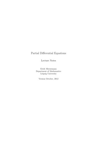
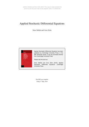
8 CHAPTER 1INTRODUCTION TO DIFFERENTIAL EQUATIONS()it is not a member of the family y 14 x2 c 2; there is no way of assigning a value tothe constant c to obtain y 0.In all the preceding examples we used x and y to denote the independent anddependent variables, respectively. But you should become accustomed to seeingand working with other symbols to denote these variables. For example, we coulddenote the independent variable by t and the dependent variable by x.EXAMPLE 4Using Different SymbolsThe functions x c1 cos 4t and x c 2 sin 4t, where c1 and c 2 are arbitrary constantsor parameters, are both solutions of the linear differential equationx 16x 0.For x c1 cos 4t the first two derivatives with respect to t are x 4c1 sin 4tand x 16c1 cos 4t. Substituting x and x then givesx 16x 16c1 cos 4t 16(c1 cos 4t) 0.In like manner, for x c 2 sin 4t we have x 16c 2 sin 4t, and sox 16x 16c2 sin 4t 16(c2 sin 4t) 0.Finally, it is straightforward to verify that the linear combination of solutions, or thetwo-parameter family x c1 cos 4t c 2 sin 4t, is also a solution of the differentialequation.The next example shows that a solution of a differential equation can be apiecewise-defined function.EXAMPLE 5You should verify that the one-parameter family y cx 4 is a one-parameter familyof solutions of the differential equation xy 4y 0 on the inverval ( , ). SeeFigure 1.1.4(a). The piecewise-defined differentiable functionyc 1xc 1yc 1,x 0xc 1,x 0(b) piecewise-defined solutionFIGURE 1.1.4y xx ,,44x 0x 0is a particular solution of the equation but cannot be obtained from the familyy cx 4 by a single choice of c; the solution is constructed from the family by choosing c 1 for x 0 and c 1 for x 0. See Figure 1.1.4(b).(a) two explicit solutionsxy 4y 0A Piecewise-Defined SolutionSome solutions ofSYSTEMS OF DIFFERENTIAL EQUATIONS Up to this point we have beendiscussing single differential equations containing one unknown function. Butoften in theory, as well as in many applications, we must deal with systems ofdifferential equations. A system of ordinary differential equations is two or moreequations involving the derivatives of two or more unknown functions of a singleindependent variable. For example, if x and y denote dependent variables and tdenotes the independent variable, then a system of two first-order differentialequations is given bydx f(t, x, y)dtdy g(t, x, y).dt(9)
1.1DEFINITIONS AND TERMINOLOGY 9A solution of a system such as (9) is a pair of differentiable functions x 1(t),y 2(t), defined on a common interval I, that satisfy each equation of the systemon this interval.REMARKS(i) A few last words about implicit solutions of differential equations are inorder. In Example 3 we were able to solve the relation x 2 y 2 25 fory in terms of x to get two explicit solutions, 1(x) 125 x2 and 2(x) 125 x2 , of the differential equation (8). But don’t read too muchinto this one example. Unless it is easy or important or you are instructed to,there is usually no need to try to solve an implicit solution G(x, y) 0 for yexplicitly in terms of x. Also do not misinterpret the second sentence followingDefinition 1.1.3. An implicit solution G(x, y) 0 can define a perfectly gooddifferentiable function that is a solution of a DE, yet we might not be able tosolve G(x, y) 0 using analytical methods such as algebra. The solution curveof may be a segment or piece of the graph of G(x, y) 0. See Problems 45and 46 in Exercises 1.1. Also, read the discussion following Example 4 inSection 2.2.(ii) Although the concept of a solution has been emphasized in this section,you should also be aware that a DE does not necessarily have to possessa solution. See Problem 39 in Exercises 1.1. The question of whether asolution exists will be touched on in the next section.(iii) It might not be apparent whether a first-order ODE written in differentialform M(x, y)dx N(x, y)dy 0 is linear or nonlinear because there is nothingin this form that tells us which symbol denotes the dependent variable. SeeProblems 9 and 10 in Exercises 1.1.(iv) It might not seem like a big deal to assume that F(x, y, y , . . . , y (n) ) 0 canbe solved for y (n), but one should be a little bit careful here. There are exceptions,and there certainly are some problems connected with this assumption. SeeProblems 52 and 53 in Exercises 1.1.(v) You may run across the term closed form solutions in DE texts or inlectures in courses in differential equations. Translated, this phrase usuallyrefers to explicit solutions that are expressible in terms of elementary (orfamiliar) functions: finite combinations of integer powers of x, roots, exponential and logarithmic functions, and trigonometric and inverse trigonometricfunctions.(vi) If every solution of an nth-order ODE F(x, y, y , . . . , y (n)) 0 on an interval I can be obtained from an n-parameter family G(x, y, c1, c 2, . . . , cn ) 0 byappropriate choices of the parameters ci, i 1, 2, . . . , n, we then say that thefamily is the general solution of the DE. In solving linear ODEs, we shall impose relatively simple restrictions on the coefficients of the equation; with theserestrictions one can be assured that not only does a solution exist on an intervalbut also that a family of solutions yields all possible solutions. Nonlinear ODEs,with the exception of some first-order equations, are usually difficult or impossible to solve in terms of elementary functions. Furthermore, if we happen toobtain a family of solutions for a nonlinear equation, it is not obvious whetherthis family contains all solutions. On a practical level, then, the designation“general solution” is applied only to linear ODEs. Don’t be concerned aboutthis concept at this point, but store the words “general solution” in the back ofyour mind —we will come back to this notion in Section 2.3 and again inChapter 4.
10CHAPTER 1 INTRODUCTION TO DIFFERENTIAL EQUATIONSEXERCISES 1.1In Problems 1 – 8 state the order of the given ordinary differential equation. Determine whether the equation is linear ornonlinear by matching it with (6).1. (1 x)y 4xy 5y cos x2. x dyd3y 3dxdx4 y 03. t 5y(4) t 3y 6y 04.d 2u du u cos(r u)dr 2dr 5.d 2ydy 1 2dxdxB6.kd 2R 2dt 2R2Answers to selected odd-numbered problems begin on page ANS-1.16. y 25 y 2; y 5 tan 5x17. y 2xy 2; y 1 (4 x 2)18. 2y y 3 cos x; y (1 sin x) 1/2In Problems 19 and 20 verify that the indicated expression isan implicit solution of the given first-order differential equation. Find at least one explicit solution y (x) in each case.Use a graphing utility to obtain the graph of an explicit solution. Give an interval I of definition of each solution .19. In Problems 21 –24 verify that the indicated family of functions is a solution of the given differential equation. Assumean appropriate interval I of definition for each solution.x2 .x x 03 In Problems 9 and 10 determine whether the given first-orderdifferential equation is linear in the indicated dependentvariable by matching it with the first differential equationgiven in (7).9. (y 2 1) dx x dy 0; in y; in x10. u dv (v uv ue u) du 0; in v; in uIn Problems 11 –14 verify that the indicated function is anexplicit solution of the given differential equation. Assumean appropriate interval I of definition for each solution.21.dPc1et P(1 P); P dt1 c1et22.dy2 2xy 1; y e xdx23. dy6 6 20y 24; y e 20tdt5 513. y 6y 13y 0; y e 3x cos 2x14. y y tan x; y (cos x)ln(sec x tan x)In Problems 15 – 18 verify that the indicated functiony (x) is an explicit solution of the given first-orderdifferential equation. Proceed as in Example 2, by considering simply as a function, give its domain. Then by considering as a solution of the differential equation, give at leastone interval I of definition.15. (y x)y y x 8; y x 4 2x 2xet dt c1e x220dyd 2y 4 4y 0; y c1e2x c2 xe2xdx2dx24. x3d 3yd 2ydy y 12x2; 2x2 2 x3dxdxdxy c1x 1 c2 x c3 x ln x 4x225. Verify that the piecewise-defined function11. 2y y 0; y e x/212. 20. 2xy dx (x 2 y) dy 0; 2x 2 y y 2 17. (sin )y (cos )y 28. ẍ 1 dX2X 1 t (X 1)(1 2X); lndtX 1y xx ,,22x 0x 0is a solution of the differential equation xy 2y 0on ( , ).26. In Example 3 we saw that y 1(x) 125 x2 andy 2(x) 125 x2 are solutions of dy dx x y on the interval ( 5, 5). Explain why the piecewisedefined functiony 125 x 125 x,2,2 5 x 00 x 5is not a solution of the differential equation on theinterval ( 5, 5).
1.1In Problems 27–30 find values of m so that the functiony emx is a solution of the given differential equation.27. y 2y 028. 5y 2y29. y 5y 6y 030. 2y 7y 4y 0In Problems 31 and 32 find values of m so that the functiony xm is a solution of the given differential equation.31. xy 2y 032. x2y 7xy 15y 0In Problems 33– 36 use the concept that y c, x ,is a constant function if and only if y 0 to determinewhether the given differential equation possesses constantsolutions.33. 3xy 5y 1034. y y 2 2y 335. (y 1)y 1DEFINITIONS AND TERMINOLOGY 1143. Given that y sin x is an explicit solution of thedyfirst-order differential equation 11 y2. Finddxan interval I of definition. [Hint: I is not the interval( , ).]44. Discuss why it makes intuitive sense to presume thatthe linear differential equation y 2y 4y 5 sin thas a solution of the form y A sin t B cos t, whereA and B are constants. Then find specific constants Aand B so that y A sin t B cos t is a particular solution of the DE.In Problems 45 and 46 the given figure represents the graphof an implicit solution G(x, y) 0 of a differential equationdy dx f (x, y). In each case the relation G(x, y) 0implicitly defines several solutions of the DE. Carefullyreproduce each figure on a piece of paper. Use differentcolored pencils to mark off segments, or pieces, on eachgraph that correspond to graphs of solutions. Keep in mindthat a solution must be a function and differentiable. Usethe solution curve to estimate an interval I of definition ofeach solution .36. y 4y 6y 1045.yIn Problems 37 and 38 verify that the indicated pair offunctions is a solution of the given system of differentialequations on the interval ( , ).37.dx x 3ydt38.d 2x 4y etdt 2dy 5x 3y;dtd 2y 4 x et;dt 2x e 2t 3e6t,x cos 2t sin 2t 15 et,y e 2t 5e6ty cos 2t sin 2t 15 et1x1FIGURE 1.1.5 Graph for Problem 4546.yDiscussion Problems39. Make up a differential equation that does not possessany real solutions.11x40. Make up a differential equation that you feel confidentpossesses only the trivial solution y 0. Explain yourreasoning.41. What function do you know from calculus is such thatits first derivative is itself? Its first derivative is aconstant multiple k of itself? Write each answer inthe form of a first-order differential equation with asolution.42. What function (or functions) do you kn
1 1 INTRODUCTION TO DIFFERENTIAL EQUATIONS 1.1 Definitions and Terminology 1.2 Initial-Value Problems 1.3 Differential Equations as Mathematical Models CHAPTER 1 IN REVIEW The words differential and equations certainly suggest solving some kind of equation that contains derivatives y, y, . . . .Analogous to a course in algebra and