WIXLIB

An Introduction to Differential EvolutionKelly Fleetwood

Synopsis Introduction Basic Algorithm Example Performance Applications

The Basics of Differential Evolution Stochastic, population-based optimisation algorithm Introduced by Storn and Price in 1996 Developed to optimise real parameter, real valued functions General problem formulation is:For an objective function f : X RD R where the feasible regionX 6 , the minimisation problem is to findx X such that f (x ) f (x) x Xwhere:f (x ) 6

Why use Differential Evolution? Global optimisation is necessary in fields such as engineering, statisticsand finance But many practical problems have objective functions that are nondifferentiable, non-continuous, non-linear, noisy, flat, multi-dimensionalor have many local minima, constraints or stochasticity Such problems are difficult if not impossible to solve analytically DE can be used to find approximate solutions to such problems

Evolutionary Algorithms DE is an Evolutionary Algorithm This class also includes Genetic Algorithms, Evolutionary Strategies andEvolutionary ctionFigure 1: General Evolutionary Algorithm Procedure

Notation Suppose we want to optimise a function with D real parameters We must select the size of the population N (it must be at least 4) The parameter vectors have the form:xi,G [x1,i,G , x2,i,G , . . . xD,i,G ] i 1, 2, . . . , N.where G is the generation number.

election Define upper and lower bounds for each parameter:UxLj xj,i,1 xj Randomly select the initial parameter values uniformly on the intervalsU[xLj , xj ]

on Each of the N parameter vectors undergoes mutation, recombination andselection Mutation expands the search space For a given parameter vector xi,G randomly select three vectors xr1,G ,xr2,G and xr3,G such that the indices i, r1, r2 and r3 are distinct

on Add the weighted difference of two of the vectors to the thirdvi,G 1 xr1,G F (xr2,G xr3,G ) The mutation factor F is a constant from [0, 2] vi,G 1 is called the donor vector

lection Recombination incorporates successful solutions from the previous generation The trial vector ui,G 1 is developed from the elements of the target vector,xi,G , and the elements of the donor vector, vi,G 1 Elements of the donor vector enter the trial vector with probability CR

RecombinationInitialisationuj,i,G 1MutationRecombinationSelection vj,i,G 1 if randj,i CR or j Irand xj,i,Gif randj,i CR and j 6 Irandi 1, 2, . . . , N ; j 1, 2, . . . , D randj,i U [0, 1], Irand is a random integer from [1, 2, ., D] Irand ensures that vi,G 1 6 xi,G

ion The target vector xi,G is compared with the trial vector vi,G 1 and theone with the lowest function value is admitted to the next generation ui,G 1 if f (ui,G 1 ) f (xi,G )xi,G 1 i 1, 2, . . . , N xi,Gotherwise Mutation, recombination and selection continue until some stopping criterion is reached

Example: Ackley’s function DE with N 10, F 0.5 and CR 0.1 Ackley’s functionrf (x1 , x2 ) 20 e 20exp 0.2!1 2(x1 x22 ) expn 1(cos(2πx1 ) cos(2πx2 ))n Find x [ 5, 5] such that f (x ) f (x) x [ 5, 5] f (x ) 0; x (0, 0)

Example: Ackley’s function15f(x)1050 550x2 5 5 4 3 2 1x1012345

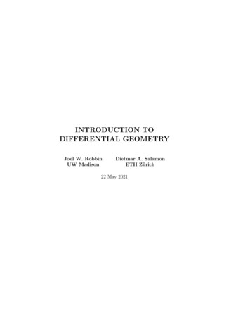
Example: Ackley’s function51441231021x2806 1 24 32 4 5 5 4 3 2 10x1123450

Example: Initialisation5432x210 1 2 3 4 5 5 4 3 2 10x112345

Example: Mutation5432x210 1 2 3 4 5 5 4 3 2 10x112345

Example: Mutation5432x210 1 2 3 4 5 5 4 3 2 10x112345

Example: Mutation5432x210 1 2 3 4 5 5 4 3 2 10x112345

Example: Mutation5432x210 1 2 3 4 5 5 4 3 2 10x112345

Example: Mutation5432x210 1 2 3 4 5 5 4 3 2 10x112345

Example: Recombination5432x210 1 2 3 4 5 5 4 3 2 10x112345

Example: Selection5432x210 1 2 3 4 5 5 4 3 2 10x112345

Example: Selection5432x210 1 2 3 4 5 5 4 3 2 10x112345

Example: Selection5432x210 1 2 3 4 5 5 4 3 2 10x112345

Example: Mutation5432x210 1 2 3 4 5 5 4 3 2 10x112345

Example: Mutation5432x210 1 2 3 4 5 5 4 3 2 10x112345

Example: Mutation5432x210 1 2 3 4 5 5 4 3 2 10x112345

Example: Mutation5432x210 1 2 3 4 5 5 4 3 2 10x112345

Example: Mutation5432x210 1 2 3 4 5 5 4 3 2 10x112345

Example: Recombination5432x210 1 2 3 4 5 5 4 3 2 10x112345

Example: Recombination5432x210 1 2 3 4 5 5 4 3 2 10x112345

Example: Selection5432x210 1 2 3 4 5 5 4 3 2 10x112345

Example: Selection5432x210 1 2 3 4 5 5 4 3 2 10x112345

Example: Generation 25432x210 1 2 3 4 5 5 4 3 2 10x112345

Example: Generation 15432x210 1 2 3 4 5 5 4 3 2 10x112345

Example: Movie Thirty generations of DE N 10, F 0.5 and CR 0.1 Ackley’s function

Performance There is no proof of convergence for DE However it has been shown to be effective on a large range of classicoptimisation problems In a comparison by Storn and Price in 1997 DE was more efficient thansimulated annealing and genetic algorithms Ali and Törn (2004) found that DE was both more accurate and moreefficient than controlled random search and another genetic algorithm In 2004 Lampinen and Storn demonstrated that DE was more accurate than several other optimisation methods including four genetic algorithms, simulated annealing and evolutionary programming

Recent Applications Design of digital filters Optimisation of strategies for checkers Maximisation of profit in a model of a beef property Optimisation of fermentation of alcohol

Further Reading Price, K.V. (1999), ‘An Introduction to Differential Evolution’ in Corne,D., Dorigo, M. and Glover, F. (eds), New Ideas in Optimization, McGrawHill, London. Storn, R. and Price, K. (1997), ‘Differential Evolution - A Simple and Efficient Heuristic for Global Optimization over Continuous Spaces’, Journalof Global Optimization, 11, pp. 341–359.

The Basics of Differential Evolution Stochastic, population-based optimisation algorithm Introduced by Storn and Price in 1996 Developed to optimise real parameter, real valued functions General problem formulation is: For an objective function f : X RD R where the feasible region X 6 , the minimisation problem is .