Transcription
The Synthetic data vaultNeha PatkiRoy WedgeKalyan VeeramachaneniCSAIL, MITCambridge, MA - 02139npatki@mit.eduLIDS, MITCambridge, MA - 02139rwedge@mit.eduLIDS, MITCambridge, MA- 02139kalyanv@mit.eduAbstract—The goal of this paper is to build a system thatautomatically creates synthetic data to enable data science endeavors. To achieve this, we present the Synthetic Data Vault(SDV), a system that builds generative models of relationaldatabases. We are able to sample from the model and createsynthetic data, hence the name SDV. When implementing theSDV, we also developed an algorithm that computes statistics atthe intersection of related database tables. We then used a stateof-the-art multivariate modeling approach to model this data. TheSDV iterates through all possible relations, ultimately creating amodel for the entire database. Once this model is computed, thesame relational information allows the SDV to synthesize data bysampling from any part of the database.Similarly, for online transactional data, one can extract thesequence of actions taken by customers, learn a hidden Markovmodel, and subsequently sample sequences from it. Thesestrategies, while important in their own right, involve modelingdata only after it has been aggregated and/or transformed witha purpose in mind. Whatever synthetic data is produced underthese conditions can only aid that same purpose—for example,users working with synthetic action sequences can only exploreand build solutions for problems that are defined over them. Toenable a multitude of data science endeavors, we challengedourselves to model the database directly, and to do so with nospecific dataset in mind.After building the SDV, we used it to generate synthetic datafor five different publicly available datasets. We then publishedthese datasets, and asked data scientists to develop predictivemodels for them as part of a crowdsourced experiment. By analyzing the outcomes, we show that synthetic data can successfullyreplace original data for data science. Our analysis indicates thatthere is no significant difference in the work produced by datascientists who used synthetic data as opposed to real data. Weconclude that the SDV is a viable solution for synthetic datageneration.In the past, several researchers have focused on statisticallymodeling data from a relational database for the purposes offeature engineering [1] or insight generation [2]. [2] laid aBayesian network over a relational data model and learned theparameters for the conditional data slices at the intersection ofthose relations. By extending these two concepts, we developa multi-level model with a different aim—not insights, butrich synthetic data. To do this, we not only have to create astatistically validated model; we also have to pay attention tothe nuances in the data, and imitate them. For instance, wetreated missing values in a number of different ways, and builtin the ability to handle categorical values and datetime values.I.I NTRODUCTIONAn end-to-end data science endeavor requires humanintuition as well as the ability to understand data and posehypotheses and/or variables. To expand the pool of possibleideas, enterprises hire freelance data scientists as consultants,and in some cases even crowdsource through KAGGLE, awebsite that hosts data science competitions. In conversationswith numerous stakeholders, we found that the inability to sharedata due to privacy concerns often prevents enterprises fromobtaining outside help. Even within an enterprise, developmentand testing can be impeded by factors that limit access to data.In this paper, we posit that enterprises can sidestep theseconcerns and expand their pool of possible participants bygenerating synthetic data. This synthetic data must meet tworequirements: First, it must somewhat resemble the original datastatistically, to ensure realism and keep problems engaging fordata scientists. Second, it must also formally and structurallyresemble the original data, so that any software written on topof it can be reused.In order to meet these requirements, the data must bestatistically modeled in its original form, so that we can samplefrom and recreate it. In our case and in most cases, that formis the database itself. Thus, modeling must occur before anytransformations and aggregations are applied. For example,one can model covariates as a multivariate distribution, andthen sample and create synthetic data in the covariates space.In this paper, we make the following contributions:1) Recursive modeling technique: We present a methodfor recursively modeling tables in the database, allowingus to synthesize artificial data for any relational dataset.We call our approach “recursive conditional parameteraggregation”. We demonstrate the applicability of ourapproach using 5 publicly available relational datasets.2) Creation of synthetic data: We demonstrate that when adataset and its schema are presented to our system (whichwe call Synthetic Data Vault), users can generate as muchdata as they would like post-modeling, all in the sameformat and structure as the original data.3) Enable privacy protection: To increase privacy protection, users can simply perturb the model parameters andcreate many different noisy versions of the data.4) Demonstration of its utility: To test whether syntheticdata (and its noisy versions) can be used to create datascience solutions, we hired 39 freelance data scientists todevelop features for predictive models using only syntheticdata. Below we present a summary of our results.Summary of results: We modeled 5 different relationaldatasets, and created 3 versions of synthetic data, both withand without noise, for each of these datasets. We hired 39
data scientists and divided them into groups to solve predictiveproblems defined over the 5 datasets. We presented differentgroups with different versions of the data, always giving onegroup the original data. For each dataset, we compared thepredictive accuracies of features generated from the originaldata to the accuracies of those generated by users who weregiven the synthetic data. Regardless of which group it camefrom, predictive accuracy for a feature is generated by executingthat feature on the original data.We found no significant statistical difference in the datascientists’ work: For 11 out of 15 comparisons ( 70%), datascientists using synthetic data performed the same or betterthan those using the original dataset.The level of engagement with synthetic data was high: Evenwithout being told that they were working with synthetic, noisydata, data scientists engaged with it just as well as they didwith the original data. Data scientists working on synthetic datawrote a total of 4313 features on the 5 datasets.The rest of the paper is organized as follows. In Section ?we justify our focus on enabling predictive modeling throughsynthetic data generation. Section III provides an overview ofour system and its different components. Section IV presentsour modeling methodology in detail. Section V presents thealgorithm to synthesize data from our model. Section VIpresents our experimental setup, results, and conclusions.II.P REDICTIVE MODELINGOrganizeSpecify StructureIDTableLearn ModelSynthesize DataNumberTableTableTableTableTableTableΦΣ [Φ-1 (F0(X0))]Fig. 1. The SDV workflow: The user collects and formats the data, specifiesthe structure and data types, runs the modeling system, and then uses thelearned model to synthesize new data.Organize: Before supplying the data to the SDV, the user mustformat the database’s data into separate files, one for each table.Specify Structure: The user must specify basic informationabout the structure of each table, and provide it as metadatafor the database. This specification is similar to a schema inan SQL database.Columns with ID information are special, because theycontain relationship information between multiple tables. If theID column of a table references an ID column of another table,the user must specify that table.Learn Model: The user then invokes the SDV’s script tolearn the generative model. The SDV iterates through tablessequentially, using a modeling algorithm designed to accountfor relationships between the tables.Having figured out how to generate synthetic data foran arbitrary database, we asked whether this could enablepredictive modeling. We chose predictive modeling, ratherthan deriving insights based on visualization and descriptiveanalytics, for several reasons: its impact, the potential towiden the foundational bottleneck of feature engineering, anda number of observations from our own past experiences:For each table, the SDV discovers a structure of dependence.If other tables reference the current one, dependence exists,and the SDV computes aggregate statistics for the other tables.The aggregate statistics are then added to the original table,forming an extended table. This extended table is then modeled.It captures the generating information for the original tablecolumns, as well as all the dependencies between tables.– When given a database, data scientists often only lookat the first few rows of each table before jumping in todefine and write software for features.– If the data relates to a data scientist’s day-to-day activities,they will first attempt to understand the fields, and thenquickly begin to write software.– A data scientist is more likely to explore data in depthafter their first pass at predictive modeling, especially ifthat pass does not give them good predictive accuracy.The SDV uses some simple optimizations to improveefficiency. It saves all the extended tables and model informationto external files, so that subsequent invocations for the samedatabase do not perform the same computations unnecessarily.Keeping these observations in mind, along with the fact thatwe can perturb the learned model to generate noisy syntheticdata, we then asked: how much noise can we tolerate? If wecan achieve a similar end result even when a lot of noise isadded, this noise could ensure better protection of the data.To demonstrate the efficacy of this process, we assembled 5publicly available datasets, created multiple synthesized sets,and employed a crowd of data scientists to build predictivemodels from these synthesized versions. We then examinedwhether there was a statistically significant difference inpredictive model performance among the sets.III.OVERVIEWOur system, which we call Synthetic Data Vault, is brokendown into four steps, as illustrated in Figure 1.Synthesize Data: After instantiating the SDV for a database,the user is exposed to a simple API with three main functions:will1) database.get tableThis returns a model for a particular table in the database. Once the table has been found,the user can use it to perform the other two functions.2) table.synth row:The synth row function bothsynthesizes rows and infers missing data.3) table.synth children:The synth childrenfunction synthesizes complete tables that reference thecurrent table. By applying this function iteratively onthe newly-synthesized tables, the user can synthesize anentire database.The results of both synth row and synth childrenmatch the original data exactly. The SDV takes steps to deleteextended data, round values, and generate random text fortextual columns. This results in rows and tables that containfully synthesized data, which can be used in place of theoriginal.
IV.G ENERATIVE M ODELING M ETHODThis section covers the technical details of the SDV’smodeling phase in the overall workflow presented in Figure 1.The goal of the generative modeling phase is to build a completemodel for the entire relational database, given only meta filesand tables. Ultimately, the SDV’s database modeling methodbuilds generative models for individual tables. However, itperforms extra computations to account for the the relationshipsbetween them, using a method called Conditional ParameterAggregation (CPA). A high-level overview is provided byFigure 2.MetadataCSVTableCPAModelExtendedtableGaussian CopulaDistributionsCovarianceFig. 2. An overview of the generative modeling process. Conditional ParameterAggregation accounts for foreign key relations across multiple tables. TheGaussian Copula process calculates the overall table model.This section is broken into five sections: Section IV-Areviews the multivariate generative modeling method we usefor a table. This corresponds to the Gaussian Copula andmodel steps in Figure 2, and provides a foundation forour work. Section IV-B describes extending the generativemodel to encompass multiple tables. This is called conditionparameter aggregation CPA. The next two sections provideadditional adjustments necessary to make the algorithms moregeneralizable. Finally, Section IV-D provides the overall logicfor applying our technique. This means recursively applyingCPA for all tables, in order to model the entire database.A. Standalone Table ModelWe define a standalone table as a set of rows and columnsthat we wish to model independently of any other data.The generative model for a standalone table encompasses allcolumns that represent numerical data,1 and it consists of: Distributions: The probability distributions of the valuesin each column Covariances: How the value of a column affects the valueof another column in the same rowThe distribution describes the values in a column, and thecovariance describes their dependence. Together, they form adescriptive model of the entire table.1) Distribution: A generative model relies on knowing thedistribution shapes of each of its columns. The shape of thedistribution is described by the cdf function, F , but may beexpensive to calculate. A simplistic estimate is to assume theoriginal distribution is Gaussian, so that each F is completelydefined by a µ and σ 2 value. However, this is not always thecase. Instead, we turn to some other common distributionsshapes that are parametrized by different values: Uniform Distribution: Parametrized by the min and maxvalues Beta Distribution: Parametrized by α and β Exponential Distribution: Parametrized by the decay λIf the column’s data is not Gaussian, it may be better to usea different distribution. In order to test for this fit, we usethe Kolmogorov-Smirnov test [3], which returns a p-valuerepresenting the likelihood that the data matches a particulardistribution. The distribution with the higher p-value is thedistribution we use to determine the cdf function. Currently, wedecide between truncated Gaussian and uniform distributions,but we provide support to add other distributions.Note that parameters represent different statistics for eachdistribution. For this reason, the SDV also keeps track of thetype of distribution that was used to model each column. Thislets the SDV know how to interpret the parameters at a laterstage. For example, if the distribution is uniform, then theparameters represent the min and max, but if it’s Beta, thenthey represent α and β.2) Covariance: In addition to the distributions, a generativemodel must also calculate the covariances between the columns.However, the shape of the distributions might unnecessarilyinfluence the covariance estimates [4].For this reason, we turn to the multivariate version of theGaussian Copula. The Gaussian Copula removes any bias thatthe distribution shape may induce, by converting all columndistributions to standard normal before finding the covariances.Steps to model a Gaussian Copula are:1) We are given the columns of the table 0, 1, . . . , n, and theirrespective cumulative distribution functions F0 , . . . , Fn .2) Go through the table row-by-row. Consider each row as avectorX (x0 , x1 , . . . , xn ).3) Convert the row using the Gaussian Copula: Y Φ 1 (F0 (x0 )) , Φ 1 (F1 (x1 )) , . . . , Φ 1 (Fn (xn ))where Φ 1 (Fi (xi )) is the inverse cdf of the Gaussiandistribution applied to the cdf of the original distribution.4) After all the rows are converted, compute the covariancematrix, Σ of the transformed values in the table.Together, the parameters for each column distribution, andthe covariance matrix Σ becomes the generative model for thattable. This model contains all the information from the originaltable in a compact way, and can be used to synthesize newdata for this table.B. Relational Table Model Truncated Gaussian Distribution: Parametrized by themean µ, variance σ 2 , min, and max valuesIn a relational database, a table may not be standalone ifthere are other tables in the database that refer to it. Thus, tofully account for the additional influence a table may haveon others, its generative model must encompass informationfrom its child tables. To do this, we developed a method calledConditional Parameter Aggregation (CPA) that specifies howits children’s information must be incorporated into the table.Figure 3 shows the relevant stage of the pipeline.1 Later, we discuss how to convert other types of data, such as datetime orcategorical, into numercial dataThis section explains the CPA method. CPA is onlynecessary when the table being processed is not a leaf table.
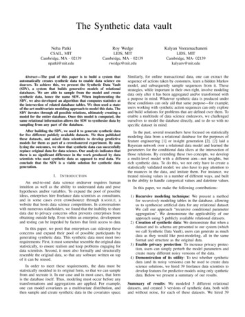
Extended tableMetadataTableCSVCPAExtendedtableID T0 T1 T2 T3 A00 A01 . C66 µ0 σ02 . σ6233Fig. 3. Aggregating data from multiple child tables creates an extended tablethat accounts for the original relations.Original columnsCurrent tableConditional dataA0 A1 A2A3333ID T0 T1 T2 T3B33A00 A01 A02Covariance: ΣA A10 A11 A12A20 A21 A22B 3 B433B BCovariance: ΣB B33 B3443443333Distributions: [(µ3, σ32), (µ4, σ42)]3333C333333DistributionsConditional parametersDistributions: [(µ0, σ02), (µ1, σ12), (µ2, σ22)]33CovariancesC5 C6C CCovariance: ΣC C55 C566566Fig. 5. The result of CPA. Every lookup for a row yields a value, such as µ5or B43 . The values form their own columns, resulting in an extended table.Original Column TypeCategoricalDatetimeNumber w/Missing ValuesCategorical w/Missing ValuesDatetime w/Missing ValuesReplaced Column(s) TypeNumberNumberNumber & CategoricalCategorical & CategoricalDatetime & CategoricalTABLE I.C ONVERSIONS THAT MUST BE MADE WHEN PRE - PROCESSING .I F MULTIPLE DATA TYPES ARE LISTED , IT MEANS THAT MULTIPLECOLUMNS ARE CREATED FROM THE ORIGINAL COLUMN .Distributions: [(µ5, σ52), (µ6, σ62)]33same database.Fig. 4. An illustration of CPA for a row in table T with primary key“33”. Tables A, B, and C refer to table T , so the lookup yields 3 setsof conditional data. Each is modeled using the Gaussian Copula, yieldingconditional parameters.Subsequently, we can use Gaussian Copula process to createa generative model of the extended table. This model not onlycaptures the covariances between the original columns, butthe dependence of the conditional parameters on the values inthe original columns. For example, it includes the covariancebetween original column T0 and derived column µ25 .This means there is at least one other table with a column thatreferences rows in the current one. CPA comprises of 4 steps:C. Pre-Processing1) Iterate through each row in the table.2) Perform a conditional primary key lookup in the entiredatabase using the ID of that row. If there are m differentforeign key columns that refer to the current table, thenthe lookup will yield m sets of rows. We call each setconditional data. Figure 4 illustrates such a lookup thatidentifies m 3 sets of conditional data.3) For each set of conditional data, perform the GaussianCopula process. This will yield m sets of distributions,and m sets of covariance matrices, Σ. We call these valuesconditional parameters, because they represent parametersof a model for a subset of data from a child, given aparent ID. This is also shown by Figure 4.4) Place the conditional parameters as additional values forthe row in the original table.2 The new columns are calledderived columns, shown in Figure 5.5) Add a new derived column that expresses the total numberof children for each parent.The extended table contains both the original and derivedcolumns. It holds the generating information for the childrenof each row, so it is essentially a table containing originalvalues and the generative models for its children. The SDVwrites a the extended table as a separate CSV file, so we donot have to recalculate CPA for subsequent invocations of the2 Somevalues repeat because Σ ΣT We drop the repeats to save space.Both Gaussian Copula and CPA assume there are no missingentries in the column, and that the values are numerical. Wheneither of assumptions is false, a pre-processing step is invoked.This step ultimately converts a column of one data type intoone or more columns of another data type, as summarized byTable I.Note that some data types might require multiple roundsof pre-processing. For example, a column that is a datetimewith missing values is first converted into two columns of typecategorical and datetime. Then, those resulting categorical anddatetime columns are further converted into number columns.1) Missing Values: Missing values in a column cannotsimply be ignored because the reasons for which they aremissing may reveal some extra information about the data. Asan example, consider a table representing people with a columncalled weight, which is missing for some rows. The reasonsfor missing data falls into one of three categories, so identifiedby the statistical analysis community [5]:– Missing not at random: The data is missing becauseof what it’s supposed to be. Perhaps people who areoverweight chose not to disclose their weight, so knowingthat the cell is missing probably means the weight is high.– Missing at random:3 The fact that the item is missing3 We realize that this is a confusing name. Think of missing at random tomean that a random subgroup decided not to supply data.
is linked with some other piece of data in that row. Forexample, perhaps a majority of females did not disclosetheir weight. So knowing that a person is female makesit more likely that the weight column will be missing.– Missing completely at random: The fact that the item ismissing tells us nothing about the structure of the rest ofthe data. For example, the database admin accidentallydeleted some of the weights, randomly (oops).In the first 2 cases, knowing that the value is missingprovides further information about the data itself. Therefore,it is important to model missing values overall. Furthermore,a high level goal of the SDV is to model and synthesize datathat mimics the format of the original. If the original data hassome missing values, the synthesized must too. Modeling thenull values solves this problem.In the final case, it is not imperative that the missing valuesare considered from a numerical perspective, but the SDV doesnot know this may be the case. Hence, even though the thirdcase is missing completely at random, the SDV must make amodel.When the SDV encounters any column that has at least 1missing value, it replaces the column with two columns:– A column of the same type, with missing values filled-inby randomly choosing non-missing values in the samecolumn.– A categorical column that contains “Yes” if the originaldata was present, and “No” if the data was missing forthat row.This solution ensures that the original column containsvalues for all rows, but also accounts for the fact that somewere originally missing.2) Categorical: Categorical columns may exist originallyin the table, or may be a result pre-processing missing values.Categorical data also cannot be modeled by the Gaussian Copulaor CPA.When it encounters a categorical column, the SDV replacesit with a numerical column containing values in the range [0, 1].To do this, it uses the following method:1) Sort the categories from most frequently occurring to least.2) Split the interval [0, 1] into sections based on the cumulative probability for each category.3) To convert a category, find the interval [a, b] [0, 1] thatcorresponds to the category.4) Chose value between a and b by sampling from a truncatedGaussian distribution with µ at the center of the interval,and σ b a6 .Figure 6 shows a visual depiction of this conversion.Note that while Gaussian distributions are completelydefined by µ and σ 2 , the same is not true for these categoricaldistributions. Instead, they require new parameters representingthe proportions ofP each of the c categories, p0 , p1 , . . . , pc with0 pi 1 and pi 1. These are the conditional parametersi4that are put in the extended table for categorical columns.4 We save p . . . p0i 1 because the last proportion pi can be calculated fromthe others.CategoricalxPr ��No”0“Yes”0.5“Maybe”0.91Fig. 6. The method that converts categorical variables to numerical data. Basedon the proportions, “No” is assigned the interval [0, 0.5]; “Yes” is assigned[0.5, 0.9], and “Maybe” is assigned [0.9, 1]. Each occupies its allocated intervalwith a Gaussian distribution.Choosing a value using a Gaussian distribution gives denseareas at the center of each interval, but ensures that the numbersare essentially different. The inverse is also easy to compute:Given a value v [0, 1], we find the interval that v correspondsto and return its category.3) Datetime: Finally, many tables contain informationcontaining times or dates that is represented as text. The SDVreplaces such columns with numerical values. This is relativelystraightforward, as any timestamp can be expressed as thenumber of seconds past Epoch (January 1, 1970). If timestamprepresents a time before Epoch, then the numerical value isnegative (number of seconds until Epoch).D. Database ModelingThis final section describes the overall system by providingcontrol logic for modeling an entire database. This consists ofapplying CPA recursively to calculate the model of the entiredatabase.We let D represent a database consisting of many tables,T . The relations between the tables are known, so we let C(T )represent the set of T ’s children, and P(T ) represent the setof T ’s parents. Finally, we assume that our logic has accessto CPA and pre-processing method we have described. Othermathematical functions include the cdf function, F , and thecovariance Σ.The CPA method works across a parent-child relationship.However, the children may have more children, so we mustapply the CPA recursively down all of the parent’s descendants.We call this recursive approach Recursive Conditional ParameterAggregation, or RCPA. Algorithm 1 provides the logic forRCPA.Algorithm 1 A recursive application of CPA to add derivedcolumns to T .1: function RCPA(T )2:for all C C(T ) do3:RCPA(C)4:T CPA(T )5:T P RE P ROCESS(T )Note that the CPA method returns the extended table. Line4 saves the extended table as T . Finally, line 5 pre-processesT to convert the values into numerical data. The base case ofthis algorithm is for leaf tables, tables where C(T ) . Suchtables are guaranteed by our non-circularity constraint.
When the SDV creates the overall model, it applies RCPAand uses the results to calculate the database model. TheSDV’s modeling algorithm calls the RCPA method on all tableswithout parents. Because RCPA is recursive, this ensures that alltables in the database ultimately go through the CPA method.Afterwards, it calculates the cdf functions, given by F , aswell as the covariances by using the Gaussian Copula for allextended tables. The logic is given in Algorithm 2.Algorithm 2 The overall modeling logic for the SDV fordatabase D.1: function SDV-M ODEL (D)2:for all T D s.t. P(T ) do3:RCPA(T )4:cdf 5:cov 6:for all T D do7:cdf cdf F (T )8:cov cov Σ(Φ 1 (F (T ))9:return cdf , covThe algorithm saves and returns all the cdf and covariancesof the tables. The cdf functions are calculated using the tablereturned by the extend function. The covariance is calculatedafter applying the Gaussian Copula to that table. Together, thecdf and covariances form the generative model for database D.When this function returns, the user can control the amountand type of data to synthesize.In summary, the overall database model saves the followingfor every table:– The extended table (calculated by Algorithm 1)– The cdfs of columns in the extended table (returned byAlgorithm 2)– The covariances of columns in the extended table (returnedby Algorithm 2)V.DATA S YNTHESISThis chapter presents the details of the last step in theSDV’s workflow: Synthesizing data based on the calculateddatabase model.We break up the synthesis into two categories:– Model-Based: The user wishes to synthesize data relyingon the model that has been computed. For example, auser may want to synthesize the entire database of theircustomer information.– Knowledge-Based: The user already has some information about the data, and wishes to synthesize the rest it.For example, the user may want to synthesize informationfor particular types of customers (female, age 22, etc.).The SDV can perform both types of synthesis. Each sectionof this chapter provides details for the two cases. The finalsection presents our API endpoints.A. Model-BasedModel-based synthesis is based on being able to sample datafrom the calculated distribution and covariances. The modelingwas learned using pre-processed numerical values that representnumbers, datetime, categories, and missing values. Once wesample from the model, we can factor in the primary key andforeign key relations to synthesize tables, and ultimately theentire database.1) Sampling Numerical Values: All numerical values can besampled from the distributions and covariances of the columns.Call the set of cdf functions F , and the covariance matrix Σ.The method to sample numerical values is given by algorithm 3.Assume that there are n columns, so that Σ F n.Algorithm 3 Sampling numerical values from distribution andcovariances of the columns.1: function S AMPLE (F , Σ)2:v random n-dimensional Guassian vector3:Find Cholesky decomposition, LLT Σ4:u Lv5:x [F0 1 (Φ(u0 )), F1 1 (Φ
II. PREDICTIVE MODELING Having figured out how to generate synthetic data for an arbitrary database, we asked whether this could enable predictive modeling. We chose predictive modeling, rather than deriving insights based on visualization and descriptive analytics, for several reasons: its impact, the potential to