Transcription
Microsoft Excel ActivityName:This activity is going to walk you through the steps needed to create a grade sheetin Microsoft Excel that will allow you to track your average for this mathematics class.Please follow the directions below carefully and see me if you need assistance!! It will bea good idea to save your work throughout the session. Saving is the same process as it inMicrosoft Word. Save all work in your student directory.1. Open a new blank Excel spreadsheet by clicking on the Microsoft Excel Icon.You will notice that a blank spreadsheet is set up in a grid pattern with each cell havingan address. This address is located in the upper-left hand corner of the screen. Thedefault starting position for the cursor box is show below as address A1.To navigate the spreadsheet you can use the arrow keys or use the mouse to click on thecell you desire to work on.2. Navigate to the cell B3 by using the mouse or arrow keys. We are going to usethis point to start making titles for each of the columns we are going to need forour gradebook.3. Enter the work “Assignment Name” in the selected cell and then press the Tabkey to move over one cell to the right. Enter “Points Possible” in this cell and then“Points Earned” in the one to the right of that. Press Tab again when you arefinished. If you completed this successfully your screen should look like this:Page 1
At this point you may notice that the words have run together and been covered becausethey are too long to fit inside the cells. Use the steps below to resize the columns to makethings fit better.4. Move the mouse cursor up until it is between the columns of B and C. If you arein the right position your mouse should chance to look like below:When the cursor changes to this you can click and hold with your mouse to resizethe column to the left of the cursor. Drag the column to the right until the word“Assignment Name” fits into the cell.5. Repeat this for each of the columns we have created. Then you can use yourmouse or cursor keys to highlight what we have worked with so far. To do thisyou have several options.a. Click and drag with the mouse until all the cells you want are highlighted.b. Start with the cursor box at one end of the set you want to highlight, holddown shift and use your arrow keys left or right until the whole section ishighlighted.c. You can also move the cursor box into position in front or behind whatyou want to highlight, press F8 and then use the cursors to move until thesection you want is highlighted.No matter what method you use, your results should look like the one below.6. Before moving on, be sure that the formatting toolbar is displayed on the screen.The formatting toolbar looks like the one below.Page 2
7. If the toolbar is not displayed:a. Go under the View menu and place your mouse over Toolbars.b. When the list expands select the Formatting toolbar my clicking on it.c. When the toolbar appears continue with the project. If you cannot get it toappear please see me before moving on.8. With our selection highlighted we are going to format our headers so they areeasily identifiable and look presentable. To do this we will be centering and thenbolding the text in the selection. To do this first click on the “Center Text” iconand then the “Bold” icon (or you can press CTRL-B to bold text). When this isdone you can see below what it turns out to be.a. Note: bolding the text may cause it to no longer fit in the cell. Resize yourcells if necessary. See step #4.9. To demonstrate one of the formatting powers of Excel we will now add anothercolumn with a title that will be used to show the percent grade earned. To do this,move the cursor to the E3 cell. Then type in the word “Percent Grade” in the celland press enter.Page 3
How does the text change after the enter key is pressed?10. Use the same method as in Step #4 to make this column the appropriate size.We now need to set up the mathematics that is going to be used in order to compute thegrades for this spreadsheet. Before moving on, check to be sure that your screen lookssimilar to the one below.In order to compute the grades for each assignment we are going to have to recall theformula for finding the percent grade given a point score. Refresh yourself with theformula below:% Grade Points Earned*100Points PossibleTake note of the fact that this formula is aligned with the columns we have already set upin our spreadsheet. To have Excel do mathematical calculations for us we need to have towork with the formula bar. The formula bar is above the column names and next to thecell address box.11. To enter a formula move the cursor box into the cell you want to results to appear.For our purposes that is the cell E4 which is the first cell in the “Percent Grade”column.Page 4
To start typing a formula you must always use the equals sign ( ) to let Excel knowwhat comes after it will be a formula and not just regular text.For our formula we are going to want to use the points possible and pointed earnedvalues to solve for our percent grade. The question we need to answer is how we aregoing to use this formula when we don’t have those values yet? We are going to usethe cell addresses we have been referencing this entire time to substitute into ourformulas. Follow the steps below to explore this.12. We need to start this off again by typing in the equals sign to let the programknow that we are going to be entering a formula. So enter the following linebelow and then we will examine the pieces of it. ( D 4 / C 4) 100% Grade Points EarnedPoints PossibleIf we break the formula down we see that we used the two cell addresses for the firstentries under Points Earned (D4) and Points Possible (C4). We substitute these inplace of actual values. This way a grade can be changed at anytime without having toredo the formula.The way things are entered now, instead of getting a numerical value like we wouldexpect we get #DIV/0!. This is an error code that lets you know there is a “divisionby zero” error. This is because we are currently pointed to blank cells, and theprogram takes them to be zeros.To fix this, lets start be inputting a grade into the gradebook.If you spreadsheet looks like the one above you can get ready to continue. If there issomething different, try to figure it out by retracing your steps or see me.If your project matches this one you have just received a grade of 5 out of 5!!!13. To enter this move the cursor box under the Assignment Name header. Type inthe name “Excel Project” as the name of the assignment and press tab. You thencan enter the value 5 and press tab again and then 5 and press tab one last time.Page 5
Until you press tab for the final time you won’t see any change in the Percent Grade.Why is this?When you’ve completed step 11 you should now have a completed grade of 100.We now need to finish off the project by looking at the total average of all thesegrades to compute the grade for the course. To do this we need to total all of thepoints earned and possible. To do this move the cursor box down to cell B30. In thisbox type “TOTALS” and then press tab to move to the next cell.14. To sum the entire column move your mouse to the formula bar and click on thefunction icon at the head of the bar.15. When you click on the formula button the Insert Function box will appear. Selectthe category “Math and Trig” and scroll down until you find the “Sum” function.Then press OK.Page 6
16. When the Function Arguments box pops up you can select what range of cells youwant to be included in your sum. You can either input the starting and stoppingbounds manually separated by a colon likeC4:C29You can also use the selection tool to pick a range of cells using the mouse.To use that method click on the icon and then click and hold the mouse tohighlight the range of cell you want and then press enter and then OK.Page 7
17. To expedite the sum process we can use a different trick to sum the point possiblecolumn. With the cursor in the D30 cell highlight up until you have selected ourfirst value (5). Then click the summation icon on the toolbar.To finish our project we need to handle getting a final grade as well as worrying abouteach assignment we enter after this one? Do we need to enter a formula for each one ofthe lines that we put an assignment on? The answer is “no.” Excel has the power to “fillin” every cell we left blank with the formula.Move the cursor box up to cell E4. Move your mouse to the lower right corner of the boxwhere there is a small “handle” on the bottom right corner. When you put your mouseover it, it will change from the pointer to aIn order to have the formula automatically fill in click on the handle in the lower rightcorner and drag down until the selection is around the E30 box and then release.What happened after the mouse was released?Page 8
You are now ready to keep track of your assignments and always know what your gradein our class is. To test to make sure the gradebook is working, complete the followingquestions before you are done.1. Enter the following assignments and grades to check that the math is workingcorrectly.Assignment NameExcel ProjectQuiz #1Homework CheckQuiz #2Exam #1Points Possible515515100What is the final grade shown?What is the grade shown for Quiz #2Page 9Points Earned51231488
2. Complete the spreadsheet by performing the following tasks/changes.a. Center all the numbers in the Points Possible and Points Earned columns.b. Bold the “TOTALS” row including the numbers.c. Bold the name of the Exam so it stands out.Print your worksheet out and attach it when you hand in the assignment.Page 10
Microsoft Word - Microsoft Excel Activity.doc Author: Jeremy Created Date: 5/1/2004 12:34:21File Size: 210KBPage Count: 10