Transcription
EXCEL BASICS: MICROSOFT OFFICE 2010GETTING STARTEDPrerequisitesWhat You Will LearnPAGE 02USING MICROSOFT EXCELOpening Microsoft ExcelMicrosoft Excel FeaturesKeyboard ReviewPointer ShapesPAGE 03MICROSOFT EXCEL BASICSPAGE 09Typing in CellsFormatting CellsInserting Rows and ColumnsSorting DataBasic FormulasCell ReferenceAutoSum and Excel EquationsCLOSING MICROSOFT EXCELSaving SpreadsheetsPrinting SpreadsheetsFinding More HelpClosing the ProgramPAGE 17To complete feedback forms, and to view our full schedule, handouts, andadditional tutorials, visit our website:cws.web.unc.eduLast Updated January 2016
2GETTING STARTEDPrerequisites:This is a class for beginning computer users. You are only expected to know how to use the mouseand keyboard, open a program, and turn the computer on and off. You should also be familiar withthe Microsoft Windows operating system.Today, we will be going over the basics of using Microsoft Excel. We will be using PC desktopcomputers running the Windows operating system. Microsoft Excel is part of the suite of programscalled “Microsoft Office,” which also includes Word, PowerPoint, and more.Please let the instructor know if you have questions or concerns before the class, or as we go along.You Will Learn How To:Find and open MicrosoftExcel in WindowsUse Microsoft Excel’smenu and toolbarReview the keyboardfunctionsUnderstand the differentpointer shapesInsert rows and columnsType in cellsFormat cellsSort your dataBasic formulasCell referencesUse AutosumSave worksheetsPrint worksheetsExit the program
3USING MICROSOFT EXCELMicrosoft Excel is an example of a program called a “spreadsheet.” Spreadsheets are used toorganize real world data, such as a check register or a rolodex. Data can be numerical oralphanumeric (involving letters or numbers). The key benefit to using a spreadsheet program is thatyou can make changes easily, including correcting spelling or values, adding, deleting, formatting,and relocating data. You can also program the spreadsheet to perform certain functions automatically(such as addition and subtraction), and a spreadsheet can hold almost limitless amounts of data—awhole filing cabinet’s worth of information can be included in a single spreadsheet. Once you create aspreadsheet, you can effortlessly print it (as many copies as you want!), save it for later modifications,or send it to a colleague via e-mail. Microsoft Excel is a very powerful calculator—This handoutcovers just a small number of its features!Microsoft Excel is available on both PCs and Macs, so what you learn in class today should beapplicable to any computer you use. The program may look slightly different depending on theversion and computer that you’re using, but Microsoft Excel will function in the same basic ways.There are other spreadsheet programs out there, including Google Spreadsheets (part of GoogleDocs), OpenOffice Calc, Apple iWorks Numbers, Lotus 1-2-3, and WordPerfect Quattro. They havemany features in common with Microsoft Excel, and you should feel free to choose any program youprefer.Opening Microsoft Excel:To get started with Microsoft Excel (oftencalled “Excel”), you will need to locate andopen the program on your computer. To openthe program, point to Excel’s icon on thedesktop with your mouse and double-click on itwith the left mouse button.If you don’t see the Excel icon on your desktop, you’llhave to access the program from the Start Menu. Click onthe button in the bottom left corner to pull up the StartMenu. You may see the Excel icon here, so click on itonce with your left button. If you still don’t see it, click on“All Programs” and scroll through the list of programs untilyou find it. It may also be located in a folder called“Microsoft Office” or something similar—it will depend onyour specific machine. Click once with your left button toopen the program.
4Excel will then open a blank page called“Book1.”This is an image of the upper-left corner ofExcel.This box features two important pieces ofinformation: the name of the file that youare currently working on (in this case,“Book1” since we have not yet renamed it)and which program you are using(“Microsoft Excel”).You will see a dark box around one of the lighter color boxes on the spreadsheet. This means that acell is selected and you will be able to enter information in that space.Microsoft Excel Features:The Title BarThis is a close-up view of the Title Bar, where file information is located. It shows the name of the file(here, “Book1,” the default title) and the name of the program (“Microsoft Excel”). You will be able toname your file something new the first time that you save it. Notice the three buttons on the right sideof the Title Bar, controlling the size and closing of the program.The Ribbon Menu SystemThe tabbed Ribbon menu system is how you navigate through Excel and access various Excelcommands. If you have used previous versions of Excel, the Ribbon system replaces the traditionalmenus.At the bottom, left area of the spreadsheet, you will find worksheet tabs. By default, three worksheettabs appear each time you create a new workbook. On the bottom, right area of the spreadsheet youwill find page view commands, the zoom tool, and the horizontal scrolling bar.
5The File MenuIn Microsoft Office 2007, there was something called the Microsoft Office Button( ) in the top left-hand corner. In Microsoft Office 2010, this has been replacedwith a tab in the Ribbon called “File.” When you left-click on this tab, a drop-downmenu appears. From this menu, you can perform the same functions as werefound under the Microsoft Office Button menu, such as: Create a new worksheet,open existing files, save files in a variety of ways, and print.
6Quick Access ToolbarOn the top left-hand side of the Title Bar, you will see several little icons above the File menu. Theselet you perform common tasks, such as saving and undoing, without having to find them in a menu.We’ll go over the meanings of the icons a little later.The Home TabThe most commonly used commands in Excel are also the most accessible. Some of thesecommands available in the Home Tab are:Font NameFont StyleFont SizeFont ColorAutoSumAlignmentSortThe Home Tab Toolbar offers options that can change the font, size, color, alignment, organizationand style of the text in the spreadsheet and individual cells. For example, the “Calibri” indicates theFONT of your text, the “11” indicates the SIZE of your text; etc. We will go over how to use all ofthese options to format your text in a little while.Each of these options expands into a menu if you left-click on the tiny down-arrow in the bottom rightcorner of the window.This tab works the exact same way as the MS Word Formatting Toolbar. The main difference is thatthe format changes will only affect the selected cell or cells, all unselected cells remain in the defaultsetting (“Calibri” font, size “11”).Formula BarThe Formula Bar is generally found below the ribbon menu. The left side denotes which cell isselected (“C5”) and the right side allows you to input equations or text into the selected cell.
7There are two ways to input information into a cell. You may either select an individual cell and typethe equation or text into the Formula Bar or type the equation or text directly into the selected cell.Equations (for example, SUM(D5 E5)) will automatically be hidden inside the cell and can only beviewed using the formula bar; the result of the equation will display in the cell.If any written text is longer than the cell width, then the spreadsheet will cover up any portion longerthan the cell width. The information will still be in the cell, you just won’t be able to see it at all times.Keyboard Review:In order to use Excel effectively, you must input commands using both the mouse and the keyboard.The above image of a keyboard should look similar to the keyboard in front of you; learning just a fewcertain keys will help to improve your efficiency in typing as well as present you with more optionswithin the program. The following is a list of commonly used keys that you may already be familiarwith:1.2.3.4.5.Backspace: This key deletes letters backwards.Delete: This key deletes letters forward.Shift: This key, when pressed WITH another key, will perform a secondary function.Spacebar: This key enters a space between words or letters.Tab: This key will indent what you type, or move the text to the right. The default indentdistance is usually ½ inch.6.Caps Lock: Pressing this key will make every letter you type capitalized.7.Control (Ctrl): This key, when pressed WITH another key, performs a shortcut.8.Enter: This key either gives you a new line, or executes a command.9.Number Keypad: These are exactly the same as the numbers at the top of the keyboard;some people just find them easier to use in this position.10.Arrow Keys: Like the mouse, these keys are used to navigate through a document orpage.
8Pointer Shapes:As with other Microsoft programs, the pointer often changes its shape as you work in Excel. Eachpointer shape indicates a different mode of operation. This table shows the various pointer shapesyou may see while working in Excel.
9MICROSOFT EXCEL BASICSTyping in Cells:Cells are the small rectangular boxes that make up the spreadsheet. The boxes are the intersectionof columns (A, B, C, etc.) and rows (1, 2, 3, etc.). To reference a cell, use the column and the rowname. For example, the cell in the first column and first row is called “A1”. All the information enteredinto an Excel spreadsheet is entered into cells.Click on a cell to begin typing in it. It is that easy! When you are finished typing in the cell, press theEnter key and you will be taken to the next cell down. You can then begin typing in that cell. You caneasily navigate around the cells using your arrow keys.Keep in mind that the Formatting toolbar in Microsoft Excel 2010 is exactly the same as the one usedfor Microsoft Word 2010. The biggest difference between the two programs is that, in Excel, theformat is set for each individual cell. So if you change the font and applied the bold option in cell C5,then this format will only be applied to cell C5. All remaining cells will remain in default mode untilthey have been changed.Sometimes you may only wish to adjust the format of one particular cell. In this case, simply selectthe cell by clicking the mouse on it and make any necessary adjustments to the font, size, style, andalignment. Those changes will not carry over when you begin typing in a new cell.Other times, you may wish to adjust the text format of a group of cells, entire rows, or entire columns.In Excel, you can choose groups of cells in rectangular units—all the cells you select must form arectangle of some kind. To select a group of cells, begin by clicking on the cell that would be in theupper-left hand corner of your rectangle. Hold down the Shift key on your keyboard and use thearrows ( , , , ) on the keyboard to expand the selection of cells, or click and drag your mouse.Once the group of cells has been selected, you can make adjustments to the font, size, style, andalignment and they will be applied to all selected cells.To select an entire row, click on the Row Number withyour mouse—note how the entire row becomeshighlighted. All formatting changes will now be applied tothe whole row.To select an entire column, click on the Column Number with your mouse—again, theentire column will become highlighted. All formatting changes will be applied to the wholecolumn.PRACTICE:Select cell A1. Type 123 in that cell and press Enter on the keyboard. Select cell C6. Type abc in thatcell and press Tab on the keyboard. Pressing Enter, Tab or left-clicking another cell will indicate toExcel that you are done typing in that cell.
10Left-click in the Formula Bar. You should now see ablinking cursor in the bar. Type hello in the bar and pressEnter. As you’re typing in the formula bar, the data appearsin the highlighted cell. Now use the Undo button in thequick access toolbar to remove “hello”. Select cell C6.Press the delete button on your keyboard to delete “abc”from that cell.Formatting Cells:The cell width and height will usually need to be adjusted to view all the information entered into acell.To adjust the cell width, move the mouse pointer in between two cell columns in thecolumn header. Hold down the left mouse button and drag the mouse left to shortenthe width or right to expand the width. Notice that all cells within the column areautomatically adjusted.Adjust the cell height using the same method. Move the mouse cursor between two rows,hold down the left mouse button and move the mouse up to decrease the height and downto increase the height.Before you begin entering data into a spreadsheet, you may already know the width and height youwant your cells to have. In this case, you can adjust all the widths and heights by doing the following:Select the “square” between Column A and Row 1. This will selectALL the cells in the spreadsheet. From the “Home” tab of the RibbonMenu, within the “Cells” box, click on “Format,” and select RowHeight. You will now be asked to enter a numerical value for height.The default value is 15, but you can enter your own height value (10,20, 25, etc.).Repeat the same steps for Column width. From the “Home” tab of the Ribbon Menu,within the “Cells” box, click on “Format,” and select Column Width. Note that thedefault value for the width is 8.43. Enter your own width value (5, 10, 15, 20, etc.).PRACTICE:In cell A1, type “1600 Penn Ave”. In cell B1, type “WashingtonDC”. You will notice that the street address is cut off and the cityblends into cell C1. If you highlight cell A1, you will see the entireaddress is still there and shows up in the formula bar. Adjust thecell width for columns A and B so you can see all the data in both cells.
11Set the row height for the entire worksheet to 20. Set the column width
Hold down the Shift key on your keyboard and use the arrows ( , , , ) on the keyboard to expand the selection of cells, or click and drag your mouse. Once the group