WIXLIB

Curve Fitting in Microsoft ExcelBy William LeeThis document is here to guide you through the steps needed to do curve fitting in Microsoft Excelusing the least-squares method.In mathematical equations you will encounter in this course, there will be a dependent variable andan independent variable. Identifying the dependent and independent variables in a mathematical equationwill help you identify what you are solving for in the equation. The independent variable is a variablewhose value determines the value of the dependent variables. Independent variable is plotted on the Xaxis, and the dependent variable is plotted on the Y-axis. Other variables may also be present in equations.These may be constants or other variables. They may be given to you or you may be required to obtainthem by performing curve fitting. The example below illustrates this point.Equation 1:y mx Cy dependent variablex independent variablem and C constantsData set:X – independent variable01020304050Y – dependent variable507090110130150Graph 1:L in e a r e q u a t io n160140120Y Data1008060402000102030X D a ta405060

When the dependent and independent variables are plotted as shown in graph 1, m and C values areobtained by adding a best fit line through the data points. m is the slope of the equation, and C is the yintercept. Adding a best-fit line in Excel can be done by using the Add Trendline.1. Add Data Set in Excel2.To graph it click on Chart Wizard button.

3. Plot the graph as XY (Scatter) with data points only. Click Finish when done.4. To add a trendline, right-click on one of the data points, then select Add Trendline

5. Select Linear Trend\Regression type.6. Click on the Options tab. Put a check on Display equation on chart and Display R-squared value onchart boxes. Click OK when done.

7. The equation for the function will be displayed on the chart as shown below.The equation displayed for the best-fit line shows m (slope) to be 2 and C (y-intercept) to be 50. Themethod shown here works well when Excel already has the built-in function, such as the function for alinear regression shown above. When the function to be used is not present in Excel (as is the case for mostfunctions you will encounter in the sciences), the method shown below should be used.

Curve fitting for the Strength-Duration DataThe equation used to fit the strength-duration data is shown below: 1V V Rh t 1 e k V stimulus strength ( dependent variable ). Plot the stimulus strength on the y-axis.VRh Rheobase. The rheobase is a constant, whose value depends on the nerve studied. You willobtain this parameter from the fit.t duration ( independent variable ). Plot the duration on the x-axis.k constant. This is also a constant. You will obtain this parameter from the fit as well.1.Input your data set as shown below.

2.Create names for k and VRh. Input the initial values for VRh and k (e.g., 1 for both Vrh and k).Then click on Insert, Name, Create. Then a new window will pop up and just click ok.3.Now you have created names for k and VRh. You can predict the strength using these constants in theequation shown below.

4.Once you have one predicted value for the first duration, double left click on the bottom right corner ofyour first predicted strength cell as shown below. This will predict the strength for all the durations.See the two figures shown below for what to expect before and after.Double left clickthere.

5.Now we have predicted the strength for all the durations. We can take the difference between theactual data and the predicted value, and calculate the square of the differenced all the predicted datapoints (e.g., strengths).6.Now we have calculated the square of the differences. We can then sum the square of the differencesby using the AutoSum button as shown below.

7.Now you have all the data for the analysis. Now click on Tools, Solver.8.A new window will open as shown below. Set the sum of diff 2 cell as your Target Cell.Click to select the target cell

Click here after you have selected thesum of diff 2 cell9.Now make the target cell Equal to Min. Under By Changing Cells, select the cells where the numericvalues of VRh and k are located as shown below.Set target cell to MinClick there to select Vrh & k

10. Now you can click on Solve and Excel will minimize the difference between the predicted strength andactual strength by changing the values of VRh and k. A new window will popup after you click solve,just click OK.11. Now plot both the actual and predicted values in Excel. You can do this by highlighting the duration,strength and predicted strength columns as shown below. Then click on the Chart Wizard button.12. Select XY scatter as the chart type and click finish.

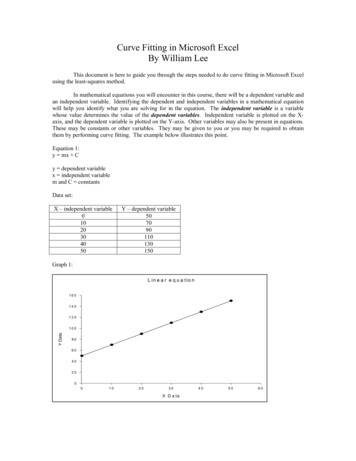
13. Now your predicted points are shown in pink and your actual values are shown in blue. Notice thepredicted values do not fall exactly on top of the actual strength. This means the predicted values arenot good.

14. To allow solver to minimize the sum of square of differences, the initial values for VRh and k have to beclose to the final predicted values. So change VRh to 0.5 and k to 0.02.15. Use solver again to solve. This is what you will get.Now you can use the predicted values to calculate the Chronaxie. This is the end of the tutorial.

Curve Fitting in Microsoft Excel By William Lee This document is here to guide you through the steps needed to do curve fitting in Microsoft Excel using the least-squares method. In mathematical equations you will encounter in this course, there will be a dependent variable and an independent variable. Identifying the dependent and independent variables in a mathematical equation will help you .