Transcription
a guide toProbability and Statistics inMicrosoft Excel Resources to support the learning of mathematics,statistics and OR in higher education.www.mathstore.ac.ukThe Statistical Education through Problem Solving (STEPS)glossarywww.stats.gla.ac/steps/glossary
Probability and Statistics in Microsoft Excel Excel provides more than 100 functions relating to probability and statistics. It also has a facility forconstructing a wide range of charts and graphs for displaying data. This leaflet provides a quick referenceguide to assist you in harnessing Excel’s statistical capability. Except where indicated, the features includedhere are available in Excel Versions 4.0 and above. Almost all the instructions here also apply to thespreadsheet facility in OpenOffice ( http://openoffice.org‐suite.com/ ); any slight variations in commandsshould be obvious to the user.Excel is not designed for statistical computing. If you require statistical analysis beyond data validation andmanipulation, tabulation, presentation and calculation of summary statistics, you are advised to use abespoke statistical package such as Minitab or SPSS.Excel has an Analysis Toolpak optional “add‐in” facility that includes macros for carrying out manyelementary statistical analyses. The instructions for installation of this add‐in vary with the version of Excel— use the Help facility in Excel for further information on this. This add‐in facility is not used in this leaflet.There are two reasons why this add‐in should be used with care: Unlike other spreadsheet functionality, which ensures that calculations automatically update in thelight of changes elsewhere in the workbook, the output from the add‐in is not dynamically linked to thesource data. Hence if any of the data change the add‐in must be run again to obtain updated output. Output from the add‐in can be misleading (see http://support.microsoft.com/kb/829252 for example).There are other commercially available add‐ins that make use of Excel’s familiar user interface butsupplement its statistical functionality. Examples include:Analyse‐it lisade.com/stattools/Using this leafletSuppose you have a sample of three data, 10.4, 11.2 and 16.4, that you have entered into cells A2:A4 on aworksheet. In Excel a function, e.g. SUM, can be applied to these data in one of four ways: SUM(10.4, 11.2, 16.4) SUM(A2, A3, A4) SUM(A2:A4) SUM(x)where x is the name attached to range A2:A4.In this leaflet, for simplicity, we have chosen to refer to namedranges. To name a range, simply highlight the range of cells, click inthe Name Box on the far left of the Formula Bar, type in the requiredname, e.g. x, then press Enter. In Excel 2007 names can be managedvia Formulas Name Manager.If you prefer not to use names then in what follows simply replace thename of the range, e.g. x, by the range address, e.g. A2:A4.
Descriptive StatisticsAssuming a sample of data in range xSample total, ΣxSample size, nSample mean, Σx/nSample variance, s2Sample standard deviation, sMean squared deviationRoot mean squared deviationCorrected sum of squares, SxxRaw sum of squares, Σx2Minimum valueMaximum valueRangeLower Quartile, Q1*Median, Q2Upper Quartile, Q3*Interquartile range, IQRKth PercentileMode SUM(x) COUNT(x) AVERAGE(x) VAR(x) STDEV(x) VARP(x) STDEVP(x) DEVSQ(x) SUMSQ(x) MIN(x) MAX(x) MAX(x)‐MIN(x) QUARTILE(x, 1) MEDIAN(x) QUARTILE(x, 3) QUARTILE(x, 3) ‐ QUARTILE(x, 1) PERCENTILE(x, K%)where K is a number between 0 and 100 MODE(x)*Note: There are several different definitions for the upper and lower quartiles, so the values calculated byExcel may not agree with your textbook or other statistical calculation tools.BoxplotSee http://www.coventry.ac.uk/ec/ nhunt/boxplot.htmGrouped Frequency DataAssuming a frequency distribution with class midpoints stored in range x and frequencies in range f:Sample size, nSample total, ΣfxSample mean, Σfx/nCorrected sum of squares, SxxSample variance, s2Sample standard deviation, s SUM(f) SUMPRODUCT(f, x) SUMPRODUCT(f, x)/SUM(f) SUMPRODUCT(f, x, x)‐SUMPRODUCT(f, x) 2/SUM(f) (SUMPRODUCT(f, x, x)‐SUMPRODUCT(f, x) 2/SUM(f))/(SUM(f)‐1) SQRT(Sample variance)Graphical RepresentationsExcel offers a wide range of chart types for displaying data. Many of these are over‐elaborate. Inparticular, 3‐D effects can be misleading and should be avoided.In Excel 2007 to construct a chart for your data:1. Select the range containing your data, including any row or column labels.2. On the main ribbon, click on the Insert tab.3. Under the Charts group of icons, select the chart type required, then the preferred chart subtype.4. Under Chart Tools on the main ribbon, use the Design, Layout and Format tabs to customise the chart.In earlier versions of Excel, select the data range and then Insert Chart to invoke the Chart Wizard.
Permutations and CombinationsNumber of different combinations of m objects selected from n objectsnCm COMBIN(n, m)Number of different permutations of m objects selected from n objectsnPm PERMUT(n, m)Standard Probability DistributionsAssuming a random variable X and constants a and bBinomialBin(n, p)P(X a) BINOMDIST(a, n, p, FALSE)P(X a) BINOMDIST(a, n, p, TRUE)GeometricGeom(p)P(X a) BINOMDIST(1, a, p, FALSE)/aP(X a) 1‐BINOMDIST(0, a, p, FALSE)PoissonPo(λ)P(X a) POISSON(a, lambda, FALSE)P(X a) POISSON(a, lambda, TRUE)
PascalPasc(n, p)P(X a) NEGBINOMDIST(a‐n, n, p)P(X a) BETADIST(p, n, a‐n 1)/BETADIST(1, n, a‐n 1)NormalN(µ, σ 2)f(a) NORMDIST(a, mu, sigma, FALSE)P(X a) NORMDIST(a, mu, sigma, TRUE)P(a X b) NORMDIST(b, mu, sigma, TRUE)‐ NORMDIST(a, mu, sigma, TRUE)P(X b) 1‐NORMDIST(b, mu, sigma, TRUE)ExponentialExpon(θ)f(a) EXPONDIST(a, theta, FALSE)P(X a) EXPONDIST(a, theta, TRUE)P(a X b) EXP(‐a*theta)‐EXP(‐b*theta)P(X b) EXP(‐b*theta)GammaGa(α, β)f(a)FALSE) GAMMADIST(a, alpha, beta,P(X a) GAMMADIST(a, alpha, beta, TRUE)P(a X b)TRUE) GAMMADIST(b, alpha, beta,‐ GAMMADIST(a, alpha, beta,TRUE)P(X b)TRUE) 1‐ GAMMADIST(b, alpha, beta,
Test Statistics for Popular Significance TestsOne sample test of a meanAssuming a sample of data in range x, drawn from a population with mean µ and standard deviation σ:H0: µ µ0 H1: µ µ0Test statistic, z (AVERAGE(x)‐mu0)/(sigma/SQRT(COUNT(x)))assuming σ knownTest statistic, t ng σ unknownOne sample test of a varianceAssuming a sample of data in range x, drawn from a population with mean µ and standard deviation σ:H0: σ2 σ02 H1: σ2 σ02Test statistic, χ2 DEVSQ(x)/sigma0 2Two sample test of difference between meansAssuming two samples of data in ranges x and y, drawn from populations with means µ1 and µ2 and equalvariances:H 0: µ 1 ‐ µ 2 c H 1: µ 1 ‐ µ 2 cEstimate the unknown common standard deviation by the pooled estimate:s SQRT((DEVSQ(x) DEVSQ(y))/(COUNT(x) COUNT(y)‐2))Test statistic, t (AVERAGE(x)‐AVERAGE(y)‐c)/(s*SQRT(1/COUNT(x) 1/COUNT(y)))Two sample test of ratio of variancesAssuming two samples of data in ranges x and y, drawn from populations with variances σ12 and σ22 :H 0: σ 12 σ 22 H 1: σ 12 σ 22Test statistic, F VAR(x)/VAR(y)Chi‐squared test of associationAssuming a two‐way contingency table of observed frequencies.H0: row factor independent of column factorH1: some association between row and column factorsThe suggested layout below for a 4x2 table can easily be modified for tables of other sizes.A1:A3:C1:G3:C8:C9:C10: SUM(C3:D6) SUM(C3:D3) SUM(C3:C6) A3*C 1/ A 1 CHITEST(C3:D6,G3:H6) (COUNT(A3:A6)‐1)*(COUNT(C1:D1)‐1) CHIINV(C8,C9)copy down to A6copy across to D1copy into G3:H6
Critical Values and P‐values for Statistical TestsThere are two approaches to conducting significance tests. Some analysts like to compare the test statisticwith the critical value for a given significance level; others prefer to calculate the P‐value corresponding tothe test statistic. Excel can be used for either method.Assuming significance level α, (typically α 5% or 0.05):Two‐tailed z‐testUpper tail critical value NORMSINV(1‐alpha/2)P‐value for given z 2*(1‐NORMSDIST(ABS(z)))Two‐tailed t‐test with v degrees of freedomUpper tail critical value TINV(alpha, v)P‐value for given t TDIST(ABS(t), v, 2)One‐tailed χ 2‐test with v degrees of freedomUpper tail critical value CHIINV(alpha, v)P‐value for given chisquared CHIDIST(chisquared, v)One‐tailed F‐test with v1 degrees of freedom inthe numerator and v2 in the denominatorUpper tail critical value FINV(alpha, v1, v2)P‐value for given F FDIST(F, v1, v2)Confidence LimitsAssuming degree of confidence 100(1‐α)% (e.g. for 95% confidence α 0.05):One‐sample statistics, with data in range xFor µ (σ known)Lower limit T(x))or AVERAGE(x)‐CONFIDENCE(alpha, sigma, COUNT(x))Upper limit AVERAGE(x) NORMSINV(1‐alpha/2)*sigma/SQRT(COUNT(x))or AVERAGE(x) CONFIDENCE(alpha, sigma, COUNT(x))For µ (σ unknown)Lower limit AVERAGE(x)‐TINV(alpha, COUNT(x)‐1)*STDEV(x)/SQRT(COUNT(x))Upper limit AVERAGE(x) TINV(alpha, COUNT(x)‐1)*STDEV(x)/SQRT(COUNT(x))For σ 2Lower limit (DEVSQ(x)/CHIINV(alpha/2,COUNT(x))‐1)Upper limit (DEVSQ(x)/CHIINV(1‐alpha/2,COUNT(x))‐1)
Two‐sample statistics, with data for the first sample in range x, and the second sample in range yFor µ x ‐ µ y (σ x known, σ y known)Lower limit RT(sigmax 2/COUNT(x) sigmay 2/COUNT(y))Upper limit AVERAGE(x)‐AVERAGE(y) NORMSINV(1‐alpha/2)* SQRT(sigmax 2/COUNT(x) sigmay 2/COUNT(y))For µ x ‐ µ y (σ x and σ y unknown but assumed equal)Estimate the unknown common standard deviation by the pooled estimate:s SQRT((DEVSQ(x) DEVSQ(y))/( COUNT(x) COUNT(y)‐2))Lower limit AVERAGE(x)‐AVERAGE(y)‐TINV(alpha,COUNT(x) COUNT(y)‐2)*s*SQRT(1/COUNT(x) 1/COUNT(y))Upper limit AVERAGE(x)‐AVERAGE(y) TINV(alpha,COUNT(x) COUNT(y)‐2)* s*SQRT(1/COUNT(x) 1/COUNT(y))For σ x2 / σ y2Lower limit DEVSQ(x)/DEVSQ(y)/FINV(alpha/2, COUNT(x)‐1, COUNT(y)‐1)Upper limit (DEVSQ(x)/DEVSQ(y)/FINV(1‐alpha/2, COUNT(x)‐1, COUNT(y)‐1)Simple Linear RegressionIn Excel Versions 5 and above, a regression line (or trendline) can be added to a scatterplot by right‐clickingon one of the plotted points and selecting Add Trendline from the shortcut menu. Both linear and a varietyof non‐linear models may be fitted to the data. The equation of the fitted model may be displayed,together with the value of the coefficient of determination, R2. There are also options to extrapolate thetrendline in either direction, or to force the trendline to have a specific intercept.The trendline approach is purely graphical. To calculate predictions, regression functions must be used.
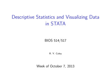
Assuming a sample of values of the independent variable in range x, and corresponding values of thedependent variable in range y:Least squares estimate of intercept, aLeast squares estimate of slope, bSxySxxSyySample covariance, Cov(x,y)Estimate of σ, sPrediction of y at x x0, ŷ a bx0 INTERCEPT(y, x) SLOPE(y, x) SUMPRODUCT(x, y)‐COUNT(x)*AVERAGE(x)*AVERAGE(y) DEVSQ(x) DEVSQ(y) COVAR(x, y)*COUNT(x)/(COUNT(x)‐1) STEYX(y, x) FORECAST(x0, y, x)Estimated standard error of individual predicted y at x x0 STEYX(y, x)*SQRT(1 1/COUNT(x) ( x0‐AVERAGE(x)) 2/DEVSQ(x))Estimated standard error of mean predicted y at x x0 STEYX(y, x)*SQRT(1/COUNT(x) ( x0‐AVERAGE(x)) 2/DEVSQ(x))CorrelationAssuming two samples of paired data in ranges x and y:Pearson product momentcorrelation coefficient, r CORREL(x, y)Rank CorrelationAssuming two samples of paired data in ranges x and y with no ties:Rank of ith value in range x RANK(INDEX(x, i), x, 1)Assuming two samples of paired data in ranges x and y with some tied values:Rank of ith value in range x (RANK(INDEX(x, i), x, 1)‐ RANK(INDEX(x, i), x, 0) COUNT(x) 1)/2Assuming that the ranges rx and ry contain the ranks of the data in x and y respectively:Spearman rank correlation coefficient, rS CORREL(rx, ry)In the example above:D2:E2:F2:F9: RANK(B2, B 2: B 7, 1) RANK(B2, B 2: B 7, 0) (D2‐E2 COUNT( B 2: B 7) 1)/2 CORREL(C2:C7, F2:F7)copy down to D7copy down to E7copy down to F7adjusted for ties
Time SeriesThe examples below refer to three years of observed quarterly data.Forecasts are made for a further four quarters (one extra year).Level onlySimple moving average period 5C4: AVERAGE(B2:B6)C14: C 11copy down to C11copy down to C17Centred moving average period 4D4: (AVERAGE(B2:B5) AVERAGE(B3:B6))/2D14: D 11copy down to D11copy down to D17Exponentially weighted moving averageE2: B2E3: G2*B3 (1‐ G2)*E2E14: E 13initial level estimatecopy down to E13copy down to E17The chart was drawn by highlighting B1:B17 and E1:E17 then using Insert Charts Line 2‐D Line.Level and constant trendC2: FORECAST(A2, B 2: B 13, A 2: A 13)copy down to C17
Level and changing trendC2:C3:D2:D3:E3:E14: B2 F2*B3 (1‐ F2)*(C2 D2) B3‐B2 G2*(C3‐C2) (1‐ G2)*D2 C2 D2 C 13 (A14‐A 13)*D 13initial level estimatecopy down to C13initial trend estimatecopy down to D13copy down to E13copy down to E17Level, changing trend and seasonalityC5:C6:D5:D6:E2:E6:F6:F14: AVERAGE(B2:B5) G 2*B6/E2 (1‐G 2)*(C5 D5) (AVERAGE(B6:B9)‐C5)/4 H 2*(C6‐C5) (1‐H 2)*D5 B2/C 5 I 2*B6/C6 (1‐I 2)*E2 (C5 D5)*E2 (C 13 (A14‐A 13)*D 13)*E10initial level estimatecopy down to C13initial trend estimatecopy down to D13copy down to E5, initial seasonal estimatescopy down to E13copy down to F13copy down to F17Version 9, 9 June 2009
Excel provides more than 100 functions relating to probability and statistics. It also has a facility for constructing a wide range of charts and graphs for displaying data. This leaflet provides a quick reference guide to assist you in harnessing Excel’s statistical capability.