Transcription
1Railway TractionJosé A. Lozano, Jesús Félez, Juan de Dios Sanz and José M. MeraUniversidad Politécnica de MadridSpain1. IntroductionThe railway as a means of transport is a very old idea. At its beginnings, it was mainlyutilised in the central European mines with different means of traction being applied. But itdid not come into general use until the invention of the steam engine. Since the 18th centuryit has developed faster and faster until in the 21st century it has become the most efficientmeans of transport for medium distances thanks to the development of High Speed.The main factors that have driven the enormous development of the railway, as any othermeans of transport, have been, and continue to be safety, speed and economy. On top of allthis, as every day passes, its environmental impact is minimum, if not zero. In the case of therailway, one of the determining factors behind its development was the type of track used,either because of its gauge or the materials used in its construction. At the start, these weremade of cast iron, but they turned out to be lacking in safety as they easily broke due to theirfragility. Towards the end of the 19th century steel began to be used as it was a less fragileand much stronger material. Nowadays, plate track is a key element in the development ofHigh Speed trains making wooden sleepers a thing of the past. The rubber track mountingswhich are currently used to support the tracks have led to enormous reductions in vibrationand noise both in the track and the rolling stock. Moreover, each country had a differenttrack gauge due to strategic reasons of commerce and defence. Today’s global markets leaveno other option but to standardise track gauges or failing that, to produce rolling stock thatcan be adapted to the different gauges quickly and automatically.The birth of the railway is linked to the birth of the steam engine, while the tremendousdevelopment of the railway in the 20th century was linked to the electrification of therailway lines. In addition, the diesel locomotive played a very important role because of itsautonomy, particularly on those lines where electrification was unviable. The rivalrybetween these three types of locomotive was long and hard with each competing to seewhich was the safest, fastest and cheapest. The first electric locomotives appeared in the lastthird of the 19th century, while the first Diesel locomotive was built at the beginning of the20th century (Faure, 2004). Diesel locomotives never reached the speeds of electriclocomotives; however, the latter require a greater investment in infrastructure to electrifythe line. As we all know, it is electric locomotives that are at the forefront of railway traction,while the Diesel locomotive is kept for some very specific uses. The final decade of the 20thcentury and the first decade of the 21st century were marked by the enormous rise in HighSpeed due to the huge leaps forward in electric locomotive technology.www.intechopen.com
4Reliability and Safety in RailwayAfter this very brief historical introduction, in this chapter, we will now focus on thedifferent types of railway traction and their importance in the development of the railway,with particular reference to safety, speed, economy and environmental impact. The basic aim isto give a detailed description of how the most generally used traction and engine systemswork in present-day railways. An analysis of the critical or least efficient points of the waythey work will lead us to discover the main criteria for optimising railway traction systems.This could be a starting point for conducting research and seeking innovations to produceever more effective and efficient traction systems. The final part of this work will suggestand justify some ideas that could be useful for improving the operating efficiency of railwaytraction systems.In order to fulfil the objectives described in the above paragraph, a methodology will beapplied that is based on the consideration of physical models that represent the behaviour ofthe railway traction systems under study, taking account of all the processes oftransformation, regulation and use of energy and even being able to recover it. Specialattention is placed on the elements that can lead to losses of energy and efficiency.Specifically, these models are developed using the Bond-Graph technique. This technique iswidely accepted for its capacity to model dynamic systems that embrace various fields ofscience and technology. Modelling is performed systematically in a way that enables all thedynamic, mechanical, electrical, electromagnetic and thermal phenomena, etc, that may beinvolved, to be taken into account. Moreover, this technique has more than proven itself tobe suited to modelling vehicular and rail systems. By taking the corresponding conceptualmodels, the Bond-Graph models are generated, and, by means of very mechanicalprocedures the behaviour equations of the dynamic systems can be found. By then takingthese behaviour equations or mathematical models, computer applications can be built tosimulate, analyse and validate the behaviour of the developed models.2. General aspects of railway tractionWhat really causes the train to accelerate or brake are the adhesion forces that appear in thewheel-rail contact. For these adhesion forces to appear, tractive or braking effort needs to beapplied to the wheels. This torque must be generated in a motor or braking system thattransforms a certain amount of energy into the required mechanical energy. These threestages form a general summary of the fundamentals of railway traction. All that needs to bedone is to develop a simple model that looks at the phenomena produced from an energypoint of view, from the moment the energy is captured until it reaches the wheel-railcontact. As a result of all this, the train accelerates or brakes.2.1 General traction equation, resistance forcesRailway traction is considered to be one of the main problems of longitudinal raildynamics (Faure, 2004; Iwnicki, 2006). It is seen as a one-dimensional problem located inthe longitudinal direction of the track, governed by the Fundamental Law of Dynamicsor Newton’s Second Law, applied in the longitudinal direction of the train’s forwardmotion: F M·awww.intechopen.com(1)
5Railway TractionWhere the term to the left of the equal sign is the sum of all the forces acting in thelongitudinal direction of the train, “M” is the total mass and “a” is the longitudinalacceleration experienced by the train. The sum of forces consists of the tractive or brakingeffort “Ft” and the passive resistances opposing the forward motion of the train, “ΣFR”, (Fig.1.-). The tractive or braking effort “Ft”, in a final instance, is the resultant of the longitudinaladhesion forces that appear in the wheel-rail contact zones, either when the train’s motorsmake the wheels rotate in the direction of forward motion, or when the braking forces act tostop the wheels rotating (in this case, these forces will obviously be negative or counter tothe direction of the train’s forward motion).Fig. 1. Longitudinal train dynamics.Let us now focus on the passive resistances that are opposing the train’s forward motion,“ΣFR”. These basically consist of five types of forces:a.b.c.d.e.Rolling resistances of the wheels.Friction between the contacting mechanical elements.Aerodynamic resistances to the train’s forward motion.Resistances to the train’s forward motion on gradients.Resistances to the train’s forward motion on curves.The phenomena associated with the appearance of the aforementioned resistances to thetrain’s forward motion are widely known (Andrews, 1986 ; Faure, 2004; Coenraad, 2001 ;Iwnicki, 2006). For this reason, we will simply present one of the most common expressionsfor modern passenger trains: FR (266,3 27,7 V 0,05168 V ) (rg 5R) (L Q)(2)Where “V” is the train’s speed in (Km/h), “rg” is the inclination of the gradient as a (o/oo),“R” is the radius of the curve in (m), “L” is the weight of the locomotives in (Tm) and “Q” isthe towed weight or the weight of the coaches in (Tm).As can be seen from equation (2), the resistances to forward motion consist of threecomponents: one constant, another that is linearly dependent on speed and another thatdepends on the speed squared. Moreover, when the train is running on a curve or agradient, the final term that is not dependent on speed needs to be added.We will now develop the Bond-Graph model, (Karnoppet alia, 2000), for the longitudinaltrain dynamics expressed in equation (1). In this model, shown in Figure 2, there are threebasic elements:a.b.The most important element is the train itself, whose longitudinal motion is representedby the Inertial port “I”. The parameter of this port is the train’s total mass, “M”.The tractive or braking efforts “Ft”. In whatever case, this is an element that suppliesenergy according to a defined force. In Bond-Graphs, these energy sources with awww.intechopen.com
6Reliability and Safety in Railwayc.defined effort are represented by the Source of Effort port “SE”. In this case, theparameter of the port is the defined effort.The third element comprises the resistances to forward motion, which are representedby the resistance port “R” in the Bond-Graph. This port will have a variable parameterso that it can satisfy the equation (2).The three ports comprising the Bond-Graph are brought together in a type “1” node, sinceall three phenomena are produced at the same speed, which is the speed of the train’sforward motion. The inertial port satisfies the following: the input force “e1” is equal to thefirst temporal derivative of the quantity of motion “P”:dPe1 (3)dtIn node “1”, given that all the bonds connected to it have the same speed, the following issatisfied: the algebraic sum of the forces is zero. Therefore, the effort “e1” equals:e1 e - e(4)Where effort “e2” is the tractive effort “Ft”, (or braking, if that is the case), and “e3” is theforce of the passive resistances (given by equation (2)).On the other hand, as we know, the Quantity of Motion “P” is equal to the product of themass “M” and the speed “V”, of the train in this case. By taking all this and entering intoequation (3), it may be easily deduced that we will reach an expression that is identical tothat shown in equation (1). In fact, it is the Inertial port “I” that resolves the fundamentalequation of dynamics given by equation (1).R : ΣFRe3SE : Fte21e1I :MFig. 2. Bond-Graph diagram of the longitudinal dynamics of the train.2.2 Tractive efforts, adhesion, powerAs already pointed out, we are not attempting to develop a complex model that takesaccount of all the driving phenomena. The main focus is to study the dynamic and energyphenomena associated with train traction or braking. For the interested reader, there is awide biography on the subject (Iwnicki, 2006).Let us now consider the steel wheel shown in Figure 3.-, moving along a longitudinal planeat a speed “V”, in contact with a steel rail and to which we apply a traction torque “T”. Alsocoming into play is the gravitational force “Mg”, where “M” is the mass suspended on thewheel and “g” is the acceleration due to gravity, the vertical reaction of the rail “N”, whichbalances the vertical forces, and the forces opposing the train’s forward motion, “ΣFR”,already mentioned in the previous section. Finally, thanks to the adhesion in the wheel-railwww.intechopen.com
7Railway Tractioncontact zone, the tangential adhesion force “Ft” appears, which satisfies the followingexpression:Ft μ N(5)Where “µ” is the so-called adhesion coefficient, whose rolling values for wheel and steel rail isdependent on temperature, humidity, dirt, etc, and particularly on speed. An expressionthat will enable us to find the value of the adhesion coefficient according to speed is thefollowing:μ μ,(6)Where “V” is the speed of the train in Km/h, and “μo” is the adhesion coefficient for zerospeed. The value of “μo” depends on the atmospheric conditions of temperature, humidity,dirt, etc, which under optimum conditions reaches a value of 0’33. Under such conditionsand V 300 km/h, we obtain: μ 0.082. Therefore, we can see that the wheel-steel rail contacthas limited possibilities when it comes to transmitting the tangential tractive or brakingefforts “Ft”,.Below is the expression used by RENFE in Spain for the adhesion coefficient, where, as iscustomary, the speed is expressed in km/h:μ μ,5 (7)Fig. 3. Tangential adhesion forces in the wheel-rail contact.Right from the beginnings of the railway the major challenge of railway traction has been toincrease the adhesion coefficient in the wheel-rail contact. Fig. 4 shows some of the adhesioncoefficient values “μo”, used. What is surprising is the high value achieved for thiscoefficient in the United States of America.www.intechopen.com
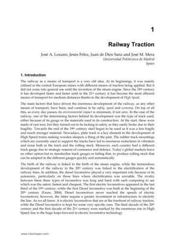
8Reliability and Safety in RailwayValues of “μo”SNCF(France)Electric monophase locomotives, multimotor bogiesElectric monophase locomotives, monomotor bogies0.330.35DB (Germany)Diesel locomotivesElectric monophase locomotives0.300.33RENFE(Spain)Diesel locomotivesClassic electric locomotivesModern electric locomotives0.22 - 0.290.270.31USASD75MAC diesel and electric locomotives0.45Fig. 4. Some values used for “μo”.Some of the methods used to improve the values of the adhesion coefficient, especiallyduring start up or acceleration, for reasons which will be made clear further on, are:a.b.c.d.Introduction of sand in the wheel-rail contact. This is the traditional method usingdevices called “sandboxes”, which are still frequently in use. However, this is a veryaggressive system regarding the wear of wheel and rail materials.Monomotor bogies that spread the tractive efforts evenly between all their shafts lead toan optimisation of the adhesion coefficient used.Drawbars that connect the locomotive chassis to the bogies in a way that thelocomotive’s weight falls on the lowest part of the bogie at a level that is as close aspossible to the wheel-rail contact. Apparently, the accelerations between the locomotivechassis and the bogie generate a force torque that aids the tractive or braking efforts,thus improving wheel-rail adhesion.Electronic anti-slip, braking and traction control systems. These are similar systems toABS, (Anti-lock Braking System), or ASR, (Anti-Slip Regulation) used in the automotiveindustry. The speed of the wheels is controlled and regulated by electronic devices sothat there is no slip between the wheels and the rails.In traction, the ideal situation is to have the maximum effort according to speed. As weknow, the power developed is the product of force and speed:Power F (8)Since the power supplied by the motor is approximately constant, the tractive effortavailable “Ft”, (given by equation (8)), dependent on the train’s speed “V”, complies with ahyperbolic-type ratio, like that shown in Figure 5.F (9)Apart from the “constant power hyperbola”, (in blue), Figure 5, also shows the maximumtractive effort curve constrained by the adhesion conditions, (in red), obtained fromequation (5) and equations (6) or (7)). If we look carefully at the constant power hyperbole, itcan be seen that at very low speed the tractive effort would tend towards infinity. However,for technical reasons, the motors are only able to supply a limited tractive effort. This iscalled “continuous tractive effort”, and appears in green.www.intechopen.com
9Railway Traction300Ft (kN), Constant power hyperboleFadh (kN), Maximum tractive effort due to wheel-rail adhesion250Ft (kN), Maximum continuous effort200150100500050100150200250300350400V (Km/h)Fig. 5. Effort-speed curves3. Railway motorsThe first railways were powered by steam engines. Although the first electric railway motorcame on the scene halfway through the 19th century, the high infrastructure costs meantthat its use was very limited. The first Diesel engines for railway usage were not developeduntil halfway through the 20th century. The evolution of electric motors for railways and thedevelopment of electrification from the middle of the 20th century meant that this kind ofmotor was suitable for railways. Nowadays, practically all commercial locomotives arepowered by electric motors (Faure, 2004; Iwnicki, 2006).Figure 6 illustrates a flow diagram for the different types of rail engines and motors mostwidely used throughout their history. The first Diesel locomotives with a mechanical orhydraulic drive immediately gave way to Diesel locomotives with electrical transmission.These locomotives are really hybrids equipped with a Diesel engine that suppliesmechanical energy to a generator, which, in turn, supplies the electrical energy to power theelectric motors that actually move the drive shafts. Although this may appear to be acontradiction in terms, it actually leads to a better regulation of the motors and greateroverall energy efficiency.www.intechopen.com
10Reliability and Safety in RailwayFig. 6. Railway engine and motor types.The major drawback of electrical traction is the high cost of the infrastructure required tocarry the electrical energy to the point of usage. This requires constructing long electricalsupply lines called “catenary”, (Figure 7). In addition, the locomotives need devices thatenable the motor to be connected to the catenary: the most common being “pantographs” orthe so-called “floaters”. In its favour, electrical traction can be said to be clean, respectful ofthe environment and efficient, as an optimum regulation of the motors can be achieved. Inthis work, we will only focus on the functioning and regulation of the most widely usedtypes of electric motors.Fig. 7. Electric railway traction: General outline, catenary and pantograph.3.1 Electric railway motorsThe most widely used electric motors for railway traction are currently of three basic types,(Lozano, 2010):1.2.3.Direct current electric motors with in-series excitation.Direct current electric motors with independent excitation.Alternating current electric motors.www.intechopen.com
Railway Traction11Direct current electric motors usually work under a 3 kV supply and alternating currentmotors under 25 kV. Direct current motors are gradually becoming obsolescent in favour ofalternating current motors. This is mainly due to maintenance problems with the directcurrent motor collectors and the better technological progress of alternating current motors.This work does not aim to provide an exhaustive development of the behaviour of electricmotors. It will only make a compilation of the equations and behaviour models of electricmotors that have already been published and accepted, particularly those that apply theBond-Graph Technique, (Karnopp, 2005; Esperilla, 2007, Lozano, 2010).Direct current electric motors (hereafter DC), are mainly made up of two components: astator or armature and a rotor or armature (see Figure 8). The stator’s mission is to generatean electric field at the core of which the rotor is inserted. This magnetic field of the stator isgenerated by windings through which an electric current is made to flow. An electriccurrent is also made to flow in the rotor. As this is immersed in a magnetic field generatedby the stator, the electric current conductor undergoes mechanical forces that cause the rotorto rotate on its shaft. The outline shown in Figure 8 corresponds to the so-called DC motorswith independent excitation, as the operating voltage of the stator and the rotor isindependent. Also, the windings of the stator and the rotor can be interconnected giving riseto two other types of DC motors:a.b.DC motors with in-series excitation, if the windings of the stator and rotor are connectedin series.DC motors with in-parallel excitation, when the windings of the stator and rotor areconnected in parallel under the same operating voltage.Firstly, we will deal with the modelling of DC motors with independent excitation and thengo on to DC motors with in-series excitation, making some slight adaptations.Fig. 8. Electromechanical circuit diagram of a DC electric motor.3.1.1 DC electric motors with independent excitationAs already indicated, Figure 8 illustrates the electromechanical outline of a DC motor withindependent excitation. Figure 9 represents the same model in a Bond-Graph using theSources of Effort “SE”, with ratios “Ue” for the stator and “Ur” for the rotor. The electricwww.intechopen.com
12Reliability and Safety in Railwaycurrent voltage “Ue”, is used to overcome the ohmic resistances “Re” in the stator circuit andto generate a magnetic field “Φ” in the winding. The ohmic resistances are represented bythe Resistance port “R” with parameter “Re”. The behaviour of the winding is frequentlyrepresented by an Inertial port. However, in this case, in order to be able to consider themagnetic losses produced in the air-gap and in the gap between the stator and the rotor, theelectrical energy reaching the winding is firstly converted into magnetic energy. Theequations governing the transformation of electrical energy into magnetic energy in thestator winding are: NM N(10)(11)Where “Φ” is the magnetic flux generated in the stator winding, “Ub” is the voltage to whichit is subjected and “Nb” is its number of turns. “M” is the induced magnetomotive force and“Ie” is the strength of the electric current in the winding. This transformation of electricalinto magnetic energy is represented in the Bond Graph by the “GY” port with a “1/Nb”ratio. The magnetic field generated by the stator winding is represented in the Bond Graphby a Compliance port “C”, in ratio to the reluctance of the magnetic field “R”, in such a waythat the relationship between the flux of the magnetic field and the magnetomotive force“M” is given by the expression:Rdt M(12)The resistance port, R, with ratio “P” represents the losses of the magnetic field produced inthe air-gap of the stator and in the gap between the stator and rotor.We will now model the electrical circuit of the rotor. In this case, the electrical energy is usedto overcome the ohmic resistances represented by the resistance port “R : Rr”, in establishingthe magnetic field of the winding represented by the Inertial port “I” with an inductanceparameter of “Lr”, and in overcoming the counter-electromotive force “E” induced by thestator’s magnetic field and which causes the rotor to rotate. All these elements described aresubjected to the same voltage as the rotor circuit “Ir”, for which reason they are connected toa “1” Junction. Due to the movement of the current “Ir” in the rotor at the core of themagnetic field generated by the stator “Φ”, mechanical forces appear that cause the rotor torotate. The equations governing the transformation of electrical into mechanical energy atthe core of the rotor (Karnopp, 2005), are: K (13)(14)Where “K” is a constant, “ ” is the motor torque generated in the rotor and “ ” is its angularvelocity. These equations for the transformation of electrical into mechanical energy arerepresented in the Bond Graph by the “MGY” port with variable ratio “K Ie”. Theconnection between the Bond Graph of the stator and the rotor is produced through thecurrent intensity “Ie”. This connection is represented by a conventional arrow with a brokenline.www.intechopen.com
13Railway TractionStatorElectrical behaviourMagnetic behaviourR : Re .1/NeGY1SE : UeC:RM0IeR : RrRotorSE :UrR:PI : LrK IeMGY1IrE RotationalmechanicalbehaviourI:J1R:μA uR : ΣFRFtV1TF : 1/rI:MBLongitudinal MechanicsFig. 9. Bond-Graph model of a DC motor with independent excitation.In the mechanical field, part of the energy is inverted to overcome the rotational inertia ofthe rotor, represented by the Inertial port “I”, the ratio of which is the moment of inertia ofthe rotor “J”; it is also inverted to overcome the friction losses in the rotor shaft supports bymeans of the Resistance port “R”, whose ratio is the viscous or Coulomb coefficient “ì”. Inthis case, these losses will be cancelled out as they are already taken into account in equation(2). As a result, what is left is the useful energy that will be inverted to power the trainthrough the drive wheels. The useful rotational energy generated by the motor is associatedwith the bond marked with the letter “A” in Figure 9, which fulfils the flow “ω”, the flow ofthe adjoining junction “1”, and the effort is the useful torque “ u”. The motor is connected tothe locomotive’s drive wheels which convert the rotational mechanical energy into linearenergy, in accordance with the following expressions: (15) (17) www.intechopen.com(16)
14Reliability and Safety in RailwayWhere “V” is the longitudinal speed of the train and “Ft” is the total tractive effort supplied bythe wheels in contact with the rails. This effort is the same as that already mentioned in section2.1 and which is shown in Figure 2. The energy transformation represented by equations (15),(16) and (17), is modelled in the Bond Graph by the Transformer port “TF:1/r”, which takesthe useful torque “ u” from the electric motor output of the bond marked with an “A” inFigure 9, and converts it into the tractive effort “Ft”. In this case the energy conversion isproduced without losses, since the mechanical losses produced are taken into account in theBond-Graph in Figure 2, without doing anything other than eliminate the Source of Effort “SE :Ft” which originally supplied the tractive effort “Ft”, and then connect the bond marked with a“B” in Figure 9 to junction “1” of the Bond-Graph in Figure 2.3.1.2 DC motors with in-series excitationDC motors a with in-series excitation are very similar to those with independent excitation,except that the circuits of the stator and the rotor are connected in series. Therefore, thecurrent flowing through both circuits is the same and is also what induces the magnetic fluxthat excites the rotor. As for the rest, everything stated concerning the independentexcitation motor is applicable to the in-series excitation motor. Figure 10 depicts the outlineof an electromechanical DC motor with in-series excitation, while Figure 11 shows itscorresponding Bond Graph.Fig. 10. Electromechanical diagram of a DC motor with in-series excitation.www.intechopen.com
15Railway TractionElectric powersupply, catenaryR : ReR : RS1/NeGY11I0SE : UElectric MotorC:RR:P1R : RrI : LrKI1RotationalMechanics I:J1MGYAR:μ uR : ΣFRFtTF : 1/rV1I:MBLongitudinal MechanicsFig. 11. Bond-Graph model of a DC motor with in-series excitation.3.1.3 Three-phase alternating current motorsThe third type of motor, which is becoming more and more used in railway traction is theasynchronous three-phase alternating current (hereafter AC) motor. This type of motor hasthe advantage of not having a collector and therefore maintenance is greatly reduced.Figure 12 shows the equivalent electrical circuit for each of the three-phase motor phases(Esperilla et al, 2007). The resistance “Re” and the winding “Le” represent the behaviour ofthe stator circuit. The Resistance “R’r” and the winding “L’r”, reduced to the stator circuit,represent the behaviour of the rotor circuit. The resistance “Rp” and the winding “Lp”represent the losses due to hysteresis produced in the air-gap and the losses due to magneticflux produced in the stator and the rotor. Finally, the resistance “R’C” is the equivalent loadresistance that models the effect of the mechanical energy produced by each motor phase,where “s” is the slip existing between the rotational velocities of the magnetic fieldgenerated by the stator and the rotor. The electrical potential dissipated through theresistance “R’C” is equivalent to the potential generated by the electric motor in each of itsphases.www.intechopen.com
16Reliability and Safety in RailwayFig. 12. Equivalent circuit of an asynchronous three-phase AC motor.Electric energysupply, catenaryMTFR : ReR : R’rR : R’c101I : LeI : L’rI : L’cR : ReR : R’rR : R’cElectric MotorMGYI:JSE : U0MTF101MGY1R:μMTFI : LeI : L’rI : L’cR : ReR : R’rR : R’c101I : LeI : L’rRotationalmechanicsMGYI : L’cFig. 13. Bond-Graph of the asynchronous three-phase motor.Figure 13 illustrates the complete Bond-Graph model of the asynchronous three-phase ACmotor. Each of the horizontal branches of the Bond-Graph models each of the phases ofthe motor, starting out from the equivalent circuit shown in Figure 4. The three phases aresubjected to an alternating current “U”, 120º out of phase using the Metatransformer portsshown to the left. The mechanical power generated by each phase is modelled by the“MGY” ports shown to the left. This rotational mechanical power is added to the “1”junction shown on the extreme right of the Bond Graph, so that it can be applied to themotor shaft modelled by the Inertial port “I” with parameter “J”. The friction losses arealso taken into account, and these are represented in the resistance port “R” withparameter “μ”.www.intechopen.com
Railway Traction174. Motor regulation and traction control techniquesIf we speak about electric motor regulation and locomotive traction control, then we alsohave to speak about power electronics. Even for the three motors dealt with in the precedingsection, the technology used in each case varies a great deal. For the reasons already statedin the previous section, at present, research conducted in this field is focused on three-phasetraction technology with asynchronous motors and a cage rotor, converters with thyristors,and, of course, control technology based on IGBT transistors and microprocessors.However, let us begin by reviewing the regulation of the two DC motors studied to then goon to the regulation of asynchronous three-phase AC motors. So as to reach a properunderstanding of the logic of the regulation techniques used in each case, we willcontinuously refer to the behaviour equations of the motors that were dealt with in theprevious section.As alr
Railway Traction José A. Lozano, Jesús Félez, Juan de Dios Sanz and José M. Mera Universidad Politécnica de Madrid Spain 1. Introduction The railway as a means of transport is a very old idea. At its beginnings, it was mainly utilised in the central European mines with diffe rent means of traction being applied. But it