Transcription
A Practical Analytic Single Scattering Model for Real Time Rendering Bo SunColumbia UniversityRavi RamamoorthiColumbia UniversitySrinivasa G. NarasimhanCarnegie Mellon UniversityShree K. NayarColumbia UniversityAbstractWe consider real-time rendering of scenes in participating media,capturing the effects of light scattering in fog, mist and haze. Whilea number of sophisticated approaches based on Monte Carlo and finite element simulation have been developed, those methods do notwork at interactive rates. The most common real-time methods areessentially simple variants of the OpenGL fog model. While easy touse and specify, that model excludes many important qualitative effects like glows around light sources, the impact of volumetric scattering on the appearance of surfaces such as the diffusing of glossyhighlights, and the appearance under complex lighting such as environment maps. In this paper, we present an alternative physicallybased approach that captures these effects while maintaining realtime performance and the ease-of-use of the OpenGL fog model.Our method is based on an explicit analytic integration of the single scattering light transport equations for an isotropic point lightsource in a homogeneous participating medium. We can implementthe model in modern programmable graphics hardware using a fewsmall numerical lookup tables stored as texture maps. Our modelcan also be easily adapted to generate the appearances of materialswith arbitrary BRDFs, environment map lighting, and precomputedradiance transfer methods, in the presence of participating media.Hence, our techniques can be widely used in real-time rendering.1(a) Clear dayIntroductionMany real-time rendering applications like games or interactivesimulations seek to incorporate atmospheric effects such as mist,fog and haze. These participating media lead to a number of qualitative effects not present in clear-day conditions (compare figure 1awith our result in figure 1c). For instance, there are often glowsaround light sources because of scattering. The shading on objectsis also softer, with specular highlights diffused out, dark regionsbrightened and shadows softer. It is critical to capture these effectsto create realistic renderings of scenes in participating media.In computer graphics, the approaches for capturing these effectsrepresent two ends in the spectrum of speed and quality. For highquality rendering, a number of Monte Carlo and finite element techniques have been proposed. These methods can model very generalvolumetric phenomena and scattering effects. However, they areslow, usually taking hours to render a single image. Significantgains in efficiency can generally be obtained only by substantialprecomputation, and specializing to very specific types of scenes.At the other extreme, perhaps the most common approach for interactive rendering is to use the OpenGL fog model, which simplyblends the fog color with the object color, based on the distance ofthe viewer (figure 1b). The fog model captures the attenuation ofsurface radiance with distance in participating media. This modelis also popular because of its simplicity—implementation requiresalmost no modification to the scene description, and the user needonly specify one parameter, β , corresponding to the scattering coefficient of the medium (density of fog). However, many qualitative e-mail:{bosun,ravir,nayar}@cs.columbia.edu; srinivas@cs.cmu.edu(b) OpenGL fog(c) Our modelFigure 1: Rendered images of a scene with 66,454 texture-mapped triangles and 4 point lights. The insets show an image for another view of thevase, with highlights from all 4 sources, to amplify shading differences. (a)Standard OpenGL rendering (without fog), (b) OpenGL fog which capturesattenuation with distance and blending with fog color, and (c) Our real-timemodel, that includes the glows around light sources, and changes to surfaceshading such as dimming of diffuse radiance (floor and wall), brighteningof dark regions (back side of pillars and vases) and dimming and diffusingof specular highlights (inset). All the visual effects in this complex scene arerendered by our method at about 20 frames per second.
Point a)ViewertrecDittecaPoint inonssimiSiossiminratTPoint SourcedressimiSnsratTrecDiPoint )onns(d)Figure 2: Diagrams showing three cases of how light travels to the viewer through the participating medium. In (a) light travels in a straight line and directlyreaches the surface and the viewer. This is essentially what previous interactive models such as OpenGL fog compute. In (b), in addition to what happens in(a), airlight scatters to the viewer and produces effects like glows around the light source. In (c), in addition to what happens in (b), airlight also scatters tothe surface and gets reflected, leading to effects such as the diffusing out of specular highlights and brightening of darker regions. In image (d), reflected raysfrom the surface also scatter to the viewer.effects are missing, such as the glows around light sources, the effect of scattering on object shading, and the ability to incorporatecomplex lighting effects like environment maps.In this paper, we take a significant step towards improving therealism of rendered images with participating media (figure 1c),while maintaining the real-time performance and ease of use ofthe OpenGL fog model. Our model can be implemented as a simple vertex or pixel shader (pseudocode in figure 13), allowing it tobe easily added to almost any interactive application. The methodcan also be applied with complex lighting, allowing environmentmapping and precomputed radiance transfer to be used interactivelywith participating media for the first time (figures 15 and 16).Figure 2 illustrates three important visual effects due to lighttransport in scattering media. In this discussion, and this paper,we assume single scattering (i.e. that light scatters at most oncein the medium), which is a common approximation in volumetricscattering and can be shown to be accurate in many common situations such as thin fog. Figure 2a corresponds to direct transmissionof light from the source or surfaces to the viewer. We can simply attenuate the clear-day radiance values based on the distance(optical thickness). This simple approach is essentially what interactive models like OpenGL fog implement. Figure 2b also includes the glows around light sources, commonly referred to asairlight [Koschmeider 1924]. Glows occur because light reachesthe viewer from different directions due to scattering in the atmosphere. Figure 2c further includes the effect of airlight on the outgoing surface radiance, leading to effects such as the spreading outof specular highlights and softening of shadows. These are important effects, usually neglected in previous interactive methods. Ourmodel renders all of the effects in figure 2c in real-time.Figure 2d illustrates the case where the surface radiance is singlescattered in addition to being attenuated, before reaching the viewpoint. On one hand, the attenuation decreases the brightness of theradiance at the surface according to the distance of the surface fromthe viewer. On the other hand, the single scattering results in slightbrightening and blurring of this surface radiance. Implementing thelatter effect requires a depth-dependent convolution. In this paper,we will only consider attenuation of surface radiance, and we willset aside a more thorough investigation of the latter effect for futurework1 . The specific technical contributions of this paper are:Explicit Compact Formula for Single Scattering:Thecommon approach to using single scattering is to numerically integrate brightness contributions while marching along the viewingray. However, this approach is too slow for interactive applications,which require an explicit formula such as the OpenGL fog model.One of the main contributions of this paper is the derivation of anexplicit compact formula for the single scattering from an isotropicpoint source in a homogeneous participating medium, by analytically integrating the single scattering equations. This airlight model(section 3) allows us to simulate effects like the glows around lightsources (figure 2b). We can also use the model to calculate the effects of scattering on the surface shading (figure 2c). These calculations are very expensive even for numerical integration, because we1 Single scattering from different surface points in the scene can partiallycompensate for the loss of brightness due to attenuation. Neglecting this canproduce consistently darker images, especially for indoor scenes.must consider incident airlight from the entire visible hemisphere.However, they can be directly implemented using our explicit surface radiance model (section 4).Implementation on Programmable Graphics Hardware:We speculate that an explicit formula for the single scattering integrals has previously not been derived because of the complexityof the calculations involved. In this paper, we reduce these difficult integrals to a combination of analytic functions that dependonly on the physical parameters of the problem, and a few lookupsof tabulated 2D functions, that have no simple analytic form, butare smooth and purely numerical—independent of the physical parameters. The numerical functions can be precomputed and storedas 2D texture maps, and the entire analytic computation and tablelookups can be implemented in simple pixel or vertex shaders inmodern programmable graphics hardware (section 5).It is alsoExtensions to Complex Lighting and BRDFs:possible to extend our airlight and surface radiance models to incorporate more complex illumination models and material properties (section 6). Mathematically, we derive a point-spread function(PSF) to represent the glow around a light source. We can convolve an environment map with this PSF to get the appearance ofa foggy scene under natural lighting. We can also use a frequencydomain spherical harmonic representation to enable rendering witharbitrary BRDFs, and add in shadows and interreflections with precomputed radiance transfer methods. This approach enables methods such as environment mapping and precomputed radiance transfer to be used with volumetric scattering effects for the first time.Our goal is to achieve interactive rendering of participatingmedia. To enable this, and derive an explicit compact expression that can be implemented in real-time, we make a numberof assumptions—isotropic point light sources, homogeneous media, the single scattering approximation, and no cast or volumetricshadows (shadows can, however, be added using precomputed lighttransport methods). More complex and general scattering effectsare certainly desirable in many situations, but are not possible toobtain at real-time rates for general scenes. On the other hand, ourmethod captures most of the important visual effects of scattering,while being very simple to add to any interactive application.2Related WorkThe literature on simulating volumetric effects is large, going backto [Blinn 1982], and we only discuss important representative papers. Most techniques are based on numerical or analytic approximations to the radiative transfer equation [Chandrasekhar 1960].Monte Carlo ray tracing methods were adapted by computer graphics researchers to render impressive effects including multiple scattering and non-homogeneous media [Kajiya and Herzen 1984; Max1994; Jensen 2001]. However, such methods can take hours to render a single image. To speed up rendering, numerical methods thatonly simulate single scattering have also been proposed [Pattanaikand Mudur 1993; Nakamae et al. 1990; Sakas 1990; Rushmeierand Torrance 1987]. However, they still require significant runningtimes, and are not suitable for interactive applications.
Hardware-accelerated numerical methods:A number ofrecent hardware-accelerated techniques can significantly decreasethe running times of numerical simulations, although they are stillusually not fast enough for many interactive applications such asgames. Dobashi et al. [2002] describe a multi-pass rendering technique that numerically integrates the single scattering equations,using graphics hardware to accumulate the results at a number ofplanes in the scene, similar to volume rendering. Harris and Lastra [2001] render clouds by including a forward scattering term inaddition to single scattering. Note that their method is geared toward the case when the viewer is far from the clouds, and theyapply a different and slower approach when the viewer and sceneare immersed inside the medium, as is the scenario in our work.These methods are intended to apply to specific phenomena likethe sky or clouds [Dobashi et al. 2002; Riley et al. 2004; Harrisand Lastra 2001]. This allows them to make use of complex tabularvolume specifications, precomputed lighting solutions or multipassrendering techniques to produce effects including inhomogeneousmedia and simple heuristics for multiple scattering. They allowfor viewpoint, and in a few cases interactive lighting variation, butusually fix the medium properties and scene specification.In contrast, our technique, while focusing on homogeneous media and single scattering, can be encapsulated in a simple shader forgeneral scenes, and allows for real time variation of the viewpoint,lighting, scattering properties of the medium, and even scene geometry and reflectance. Another major benefit of our method is that itaddresses the effects of scattering on surface shading (figure 2c)and complex lighting like environment maps. These effects are notincluded in previous methods because they are difficult to numerically simulate efficiently, requiring an integration over all incidentscattered lighting directions at each surface point.Analytically based methods: The diffusion approximation foroptically thick media was applied to subsurface scattering [Stam1995; Jensen et al. 2001]. An analytic form for the single scatteringterm was also derived by Hanrahan and Krueger [1993]. However,the problem we are solving is very different from that of subsurface scattering, where the light sources and viewer are outside themedium. In our case, both the sources and viewer are immersedinside the medium. Also, unlike in the case of diffusion, we areinterested in strongly directional effects like glows around sources.Analytic expressions for airlight with directional light sources,based on the derivation by Koschmeider [1924], are used frequentlyfor rendering skies [Preetham et al. 1999; Hoffman and Preetham2003; Narasimhan and Nayar 2002]. However, our focus is different. We wish to derive an analytic model with “near-field” pointsources, which is a significantly more complex lighting situation ascompared to distant lighting (collimated beams).Analytic expressions for the glows around point light sourcesinside homogeneous media have also been derived [Max. 1986;Biri et al. 2004; Narasimhan and Nayar 2003]. Therefore, thosemethods could be used to render glows in real time. However, itis not clear how to extend them to a complete real-time renderingsystem that also considers the effects of airlight on surface shading,or handles complex environment map lighting. Furthermore, theirderivations involve approximations that are not feasible in severalcommon rendering scenarios. For instance, the model derived byMax [1986] does not take into account attenuation. Biri et al. [2004]use a polynomial approximation to single scattering which resultsin inaccurate glows along viewing directions near the source. Themultiple scattering model in [Narasimhan and Nayar 2003] is notstrictly valid when objects are present in the medium, especiallynear the sources (as is generally true in most common scenes), or foroptically thin media. Further, the integration required for surfaceradiance cannot be computed analytically or simulated numericallyat interactive rates.3The Airlight ModelIn this section, we will derive an explicit model for the single scattered radiance at a viewer, due to an isotropic point light source,assuming that both the viewer and the source are immersed in a homogeneous scattering medium. Consider the scenario illustrated ins, v, pγDsvDvpDspTsvTvpTspβαxdI0frSubscripts for Source, Viewer, surface PointAngle between light source and viewing rayDistance between source and viewerDistance between viewer and closest surface pointDistance between source and surface pointOptical thickness between source, viewer (β Dsv )Optical thickness between viewer, surface point (β Dvp )Optical thickness between source, surface point (β Dsp )Scattering coefficient of the participating mediumAngle of scatteringDistance along the ray from viewer (integration variable)Distance of single scattering from light sourceRadiant intensity of point light sourceBRDF of surfaceFigure 3: Notation used in our derivations.Point Source, sdDsvViewer, vãxDvpáSurfacePoint, pFigure 4: Diagram showing how light is scattered once and travels from apoint light source to the viewer.figure 4 (the notations used are indicated in figure 3). The pointlight source has a radiant intensity I0 and is at a distance Dsv fromthe view point, making an angle γ with the viewing direction. Theradiance, L, is composed of the direct transmission, Ld , and thesingle scattered radiance or airlight, La ,L Ld La .(1)The direct term Ld simply attenuates the incident radiance from apoint source (I0 /D2sv ) by an exponential corresponding to the distance between source and viewer, and the scattering coefficient2 β ,Ld (γ , Dsv , β ) I0 β Dsve· δ (γ ),D2sv(2)where the delta function indicates that for direct transmission, wereceive radiance only from the direction of the source (no glows).3.1The Airlight IntegralWe focus most of our attention on the airlight La . The standard expression [Nishita and Nakamae 1987] is given by an integral alongthe viewing direction,La (γ , Dsv , Dvp , β ) Z Dvp0β k(α ) ·I0 · e β d β x·edx ,d2(3)where Dvp is the distance to the closest surface point along theviewing ray or infinity if there are no objects in that direction, andk(α ) is the particle phase function. The exponential attenuationcorresponds to the total path length traveled, d x. The two parameters d and angle α in the integrand depend on x. In particular, d is2 When there is light absorption in addition to scattering, β is called theextinction coefficient and is given by the sum of the scattering and absorption coefficients. In this paper, we simply refer to β as the scattering coefficient, and it is straightforward to include absorption in our models.
0.3FFractional 0.15vResolution010.5054u2512Figure 5: 3D plot of special function F(u, v) in the range of 0 u 10 and0 v π2 . The plot shows that the function is well-behaved and smooth andcan therefore be precomputed as a 2D table. As expected from the definitionin equation 10, the function decreases as u increases, and increases as vincreases. The maximum value in the plot above therefore occurs at (u 0, v π2 ). Also note from equation 10, that for u 0, there is no attenuationso the function is linear in v.given by the cosine rule asqd D2sv x2 2xDsv cos γ .2561286432168Figure 6: Accuracy of the airlight model. The plots show the error (versusnumerically integrating equation 5) as a function of the resolution for the2D tables for F(u, v). We report the fractional error, normalizing by the total airlight over the hemisphere. The error for each resolution is averagedover 40000 parameter values of β , Dsv , Dvp and γ . Bilinear (red) and nearest neighbor (green) interpolation is used to interpolate F(u, v) at non-gridlocations of the indices (u, v). The plots clearly indicate the high accuracyof our compact formula, and that a 64 64 table for F(u, v) suffices for amaximum error of less than 2%.0.30.08Fractional RMS error(4)Fractional RMS error0.250.06Let us now substitute equation 4 into equation 3. For now, wealso assume the phase function k(α ) is isotropic and normalizedto 1/4π (our approach can also be generalized to arbitrary phasefunctions—see appendix D on CDROM). In this case, 2 2Zβ I0 Dvp e β Dsv x 2xDsv cos γ β xdx .La (γ , Dsv , Dvp , β ) ·e4π 0 D2sv x2 2xDsv cos γ(5)We refer to this equation as the airlight single scattering integraland next focus on simplifying it further to derive an explicit form.3.2Solution to the Airlight IntegralWe take a hybrid approach to solve equation 5. The key result isthat this integral can be factorized into two expressions—(a) an analytic expression that depends on the physical parameters of thescene and (b) a two-dimensional numerically tabulated function thatis independent of the physical parameters. Essentially, this factorization enables us to evaluate the integral in equation 5 analytically.A high-level sketch of the derivation is given below and detailedsimplifications are included in appendix A.STEP 1. Reducing the dimensions of the integral: Sincethe integral in equation 5 depends on 4 parameters, our first stepis to apply a series of substitutions that reduce the dependency ofthe integrand to only one parameter. For this, we first write theexpressions in terms of optical thicknesses T β D and t β x.In most cases, this eliminates the separate dependence on both βand the distance parameters, somewhat reducing the complexity,and giving us a simpler intuition regarding the expression’s behavior. Then, we combine the dependence on Tsv and γ by making thesubstitution z t Tsv cos γ , to obtain 222Zβ 2 I0 Tsv cos γ Tvp Tsv cos γ e z z Tsv sin γedz.La (γ , Tsv , Tvp , β ) 4π Tsv cos γTsv2 sin2 γ z2(6)Now, the integrand really depends on only one physical parameterTsv sin γ , beginning to make the computation tractable.It is possible to further simplify equation 6, as described in appendix A. To encapsulate the dependence on the physical parameters of the problem, we define the following two auxiliary expressions, corresponding respectively to the normalization term outsidethe integrand, and the single physical parameter in the 52025Figure 7: Comparison of the airlight model with a standard Monte Carlosimulation that includes multiple scattering. The plots show the relativeRMS error between the two methods for the case of isotropic phase function. [Left] The low RMS errors show that our model is physically accurate(less than 4% error) for optically thin media (Tsv 2). [Right] From thisplot, it is evident that multiple scattering becomes more important as optical thickness increases. However, the actual errors grow slowly and arestill low for a wide range of optical thicknesses (Tsv 10). It is also interesting to note that for very high optical thicknesses (Tsv 20), attenuationdominates over scattering and once again the RMS errors decrease.Tsv sin γ :A0 (Tsv , γ , β ) A1 (Tsv , γ ) β 2 I0 e Tsv cos γ2π Tsv sin γTsv sin γ .(7)(8)It is then possible to derive, as shown in appendix A, thatZLa A0 (Tsv , γ , β )π4 12 arctanγ /2Tvp Tsv cos γTsv sin γexp[ A1 (Tsv , γ ) tan ξ ] d ξ .(9)Although equation 9 might seem complicated, it is really in asimplified form. We already have simple analytic expressions forA0 and A1 . Further, the function A1 is a numerical constant as faras the integration is concerned.STEP 2. Evaluating the integral using a special function:To encapsulate the key concepts in the integrand of equation 9, wedefine the special function,F(u, v) Z v0exp[ u tan ξ ] d ξ .(10)
Figure 8: The images show glows around three identical point light sources (street lamps) at different distances from the viewer. From left to right, we showthree different values of the scattering coefficient β (β 0, 0.01, 0.04). Larger values of β correspond to larger optical thicknesses Tsv . We clearly see theeffect of greater glows for larger β . Also, the radiance from farther light sources is attenuated more in each individual image, resulting in smaller glows forthe farther lights. In the fourth (rightmost) image, we show a different view with β 0.04, where all the light sources are approximately equidistant, with theresult that they have similar glows. (The shading on the surfaces is computed using the surface radiance model in section 4.)Unfortunately, there exists no simple analytic expression forF(u, v). However, the function is a well behaved 2D function asshown in figure 5. Therefore, we can simply store it numericallyas a 2D table. This is really no different from defining functionslike sines and cosines in terms of lookup tables. In practice, we willuse texture mapping in graphics hardware to access this 2D table.Note that F(u, v) is purely numerical (independent of the physicalparameters of the problem), and thus needs to be precomputed onlyonce.Finally, we can obtain for La (γ , Tsv , Tvp , β ),hTvp Tsv cos γπ 1γ iLa A0 F(A1 , arctan) F(A1 , ) , (11)4 2Tsv sin γ2where we have omitted the parameters for La , A0 and A1 for brevity.In the important special case of Tvp , corresponding to noobjects along the viewing ray, we get La (γ , Tsv , , β ) ashπγ iLa A0 (Tsv , γ , β ) F(A1 (Tsv , γ ), ) F(A1 (Tsv , γ ), ) . (12)22In summary, we have reduced the computation of a seeminglycomplex single scattering integral in equation 5 into a combination of an analytic function computation that depends onthe physical parameters of the problem and a lookup of a precomputed 2D smooth function that is independent of the physical parameters of the problem. In the rest of the paper, we willdemonstrate several extensions and applications of our model.3.3Accuracy of the Airlight ModelWe first investigate the accuracy of our analytic model as comparedto numerically integrating equation 5. Figure 6 shows plots of themean error in La as a function of the resolution of the 2D numericaltable for the special function F(u, v). We use interpolation to evaluate F(u, v) at non-grid locations for the indices (u, v) (bilinear andnearest neighbor interpolations are shown in figure 6). For eachresolution, the error computed is averaged over 40000 sets of parameter values for β , Dsv , Dvp , γ . The error bars in the figure showthe standard deviation of the errors. The plots indicate that even alow resolution 64 64 table suffices to compute F(u, v) accurately,with a maximum error of less than 2%. As expected, bilinear interpolation performs better, but, for faster rendering, one can usenearest neighbor interpolation with only a small loss in accuracy.We also validate the accuracy of the single scattering assumptionin our airlight model. Figure 7 shows the relative RMS errors between glows around light sources computed using our model and astandard volumetric Monte Carlo approach that takes into accountmultiple scattering as well. The Monte Carlo simulation took approximately two hours to compute each glow, whereas our explicitmodel runs in real-time. The comparison was conducted for opticalthicknesses over a wide range Tsv (0.25, 25) and Tvp (0.5, 50),which covers almost all real situations. As expected, for opticallythin media (Tsv 2), our model is very accurate (less than 4% relative RMS error). Interestingly, even for greater optical thicknesses(Tsv 2), the error only increases slowly. Thus, our single scattering model may be used as a viable approximation for most commonreal-time rendering scenarios, such as games.3.4Visual Effects of the Airlight ModelThe dependence of the model on the viewing direction γ and thedistance of the source from the observer Dsv , predicts visual effectslike the glows around light sources and the fading of distant objects. As discussed above, these effects are physically accurate forthin fog (low β and T ), and qualitatively reasonable in other cases.In figure 8, we also see how these glows change as a function ofthe medium properties (the scattering coefficient β ) and distanceto the sources. As β increases, we go from no glow (β T 0)to a significant glow due to scattering. The differences in the 3light sources should also be observed. The farther lights are attenuated more, and we perceive this effect in the form of reduced glowsaround more distant sources. The final (rightmost) image in figure 8shows a different viewpoint, where the sources are at approximatelythe same distance, and the glows therefore look the same.4The Surface Radiance ModelIn this section, we discuss the effects of airlight on the outgoingsurface radiance. Consider the illustration in figure 9, where anisotropic point light source s illuminates a surface point p. We willcalculate the reflected radiance at the surface. To get the actual appearance at the viewer, we need to attenuate by exp[ Tvp ] as usual,where Tvp is the optical thickness between viewer and surface point.The reflected radiance L p is the sum of contributions, L p,d andL p,a , due to direct transmission from the source, and single scattered airlight from the source respectively,L p L p,d L p,a .(13)The direct transmission corresponds to the standard surface reflectance equation, only with an attenuation of exp[ Tsp ] added because of the medium, where Tsp is the optical thickness between thesource and the surface point:L p,d I0 e Tspfr (θs , φs , θv , φv ) cos θs ,D2sp(14)where fr is the BRDF, (θs , φs ) is the direction to the source, andtherefore also the incident direction, and (θv , φv ) is the viewing direction. All angles are measured with respect to the surface normal,in the local coordinate frame of the surface.4.1The Surface Radiance IntegralOn the other hand, the single-scattered radiance L p,a is more complicated, involving an integral of the airlight (La from equation 12)over all incident direction
Hence, our techniques can be widely used in real-time rendering. 1 Introduction Many real-time rendering applications like games or interactive simulations seek to incorporate atmospheric effects such as mist, fog and haze. These participating media lead to a number of quali-tative effe