WIXLIB

3.2.1 Isotropic caseWhen all atoms vibrate with the same amplitude in all directions isotropic case, U ij (n) is proportional to the unit matrix andW (q, n) Un q 2(15)With this, we obtain the general expression for the X-ray structure factor in the isotropiccaseF (q) r0Pnfn (q)e iq·rn e Un q2(16)A very similar expression is found for the coherent neutron factor in the isotropic caseF (q) iq·rn Un q 2en bn eP(17)3.2.2 General (anisotropic) caseA few words here for the general case: anisotropic vibrations are actually very common, sinceatoms tent to vibrate more in the direction perpendicular to the bonds connecting them. In thefirst approximation, the average scattering density can be approximated by a positive-definitequadratic form, known as a thermal ellipsoid. It is rather intuitive that these thermal ellipsoidsmust be constrained by symmetry — in other words, if the atom is on a mirror plane, one of theprincipal axes of the ellipsoid must be orthogonal to the plane, etc. When one takes into accounthe site symmetry, therefore, it transpires that only certain components of U ij (n) are allowedon specific sites, and relations are set between components within each U-tensor and betweenU-tensors on symmetry-related sites.3.2.3 Temperature dependence of the Debye-Waller factorsAs we have seen in the previous sections, the Debye-Waller factor is related to the amplitude ofthe vibration and therefore both to the phonon spectrum and to the tremperature. It can be7

shown (see [1] vol 1 p 108-110) that for an isotropic, monoatomic solid of atomic mass M theexpression for W is: 2 q 2W (q, T ) 4MZdωZ(ω)1coth( ωβ)ω2(18)where Z(ω) is the phonon density of states and β 1/kB T .Here we report the result for a single oscillator (Einstein model), where Z(ω) δ(ω ωE ):WE (q, T ) 1 2 q 2coth( ωE β)4MωE2(19)In spite of its simplicity, eq. 19 is often employed to fit the temperature dependence of theDebye-Waller factors.4Laue and Bragg equationsThe δ function in eq. 8 implicitly contains the geometrical conditions for observing scatteringfrom a single crystal, which are traditionally named Laue equations 1 :q ha kb lc (20)q · a1 (kf ki ) · a1 2πhq · a2 (kf ki ) · a2 2πkq · a3 (kf ki ) · a3 2πl(21)where h, k and l are the Miller indices that we have already encountered.The Laue equations are nothing but a re-statement of the fact that q must be a RL vectorA second important relation can be obtained by considering the modulus of the scattering vector,for which, as we have already seen (fig. 1 and eq. 22 are reproduced here for convenience):1Throughout this part of the course, we will employ the convention that q is the change of wavevector of theparticle or photon, so q kf ki . the convention q ki kf identifies q with the wavevector transferred to thecrystal, and is widely employed particularly in the context of inelastic scattering8

Figure 1: Scattering triangle for elastic scattering.q q 4π sin θλ(22)2πq(23)The quantityd is known as the d-spacing. From eqs. 22 and 23 we obtain the familiar formulation of Bragg’slaw:2d sin θ λ(24)As shown in Appendix I, the d-spacing can be identified with the spacing between familiesof lattice planes perpendicular to a given RL vector.5Geometries for diffraction experimentsIn general terms, the experimental apparatus to perform a diffraction experiment on a singlecrystal or a collection of small crystals (powder diffraction) will consist of An incident beam, which can be monochromatic or polychromatic. The divergence of theincident beam is of course an important parameter, in that it determines the uncertainty9

on the Bragg angle 2θ. Various focussing schemes are possible to increase the flux on thesample or at the detector position whilst limiting the loss of resolution. A sample stage, which enables the sample to be oriented (typically a simple uniaxial rotator for powder diffraction, a Eulerian cradle or analogous arrangements for single crystalexperiments). The sample stage also incorporates the sample environment to control avariety of physical (P , T , H.) and/or chemical parameters. A detector, which includes a detector of photons or particles. Many technologies are available(gas tube, scintillator, CCD, solid-state.), depending on the type of radiation, detectorcoverage and resolution required. This is normally mounted on a separate arm, enabling the2θ angular range to be varied. On the detector arm, one often finds other devices, such asas analyser crystal and/or receiving slits to define the angular divergence of the scatteredbeam and, in the case of the analyser, to reject parasite radiation due to fluorescence.In this section, we will focus on two among the most important important geometries for diffraction experiments: the single-crystal 4-circle diffractometer and the Debye-Scherrer powderdiffractometer. Several other geometries are described in Appendix II. In their simplest form,both these geometries employ a point detector, with a spatial resolution defined by a set ofvertical and horizontal slits. Early diffractometers made extensive use of photographic film.Modern single-crystal and powder diffractometers generally employ a pixillated area detector.As an introduction to each method, we will describe two important geometrical constructions:the Ewald construction (most useful for single-crystal experiments) and the Debye-Scherrerconstruction (for powder diffraction).5.1 Single-crystal diffraction5.1.1 The Ewald constructionAs we have seen, the scattering cross section for a single crystal is a series of delta functionsin reciprocal space, centred at the nodes of the reciprocal lattice. When a single crystal is illuminated with monochromatic radiation, the scattering conditions are satisfied only for particularorientations of the crystal itself — in essence, the specular (mirror-like) reflection from a familyof lattice planes must satisfy Bragg law at the given wavelength.With monochromatic radiation, for a generic crystal orientation, no Bragg scattering willbe observed at all.The German physicist Paul Peter Ewald devised a very useful graphical construction, knownas the Ewald construction, to establish the orientation of the crystal axes with respect to the10

incident beam required to satisfy the scattering conditions. Although largely superseded as apractical calculation device, Ewald construction is of great pedagogical value to illustrate singlecrystal scattering (not exclusively with monochromatic radiation), and we will illustrate it herein some detail.The Ewald construction is made in the following steps (see fig. 2)1. A reciprocal lattice plane, coinciding with the scattering plane, is drawn first, in anarbitrary orientation.2. The incident beam direction is then marked with a line through the origin of the RL.3. The incident wavevector ki is drawn with an arrow, with the point at the origin ofthe RL and of the appropriate length to be at the correct scale (same conversion, say,between Å 1 and cm 1 ) with respect to the RL.4. A circle centred on the tail of the arrow, and passing through the origin of the RL isdrawn. In a full 3-dimensional construction, the circle would be replaced with a sphere,so they are both known as the Ewald sphere.5. Scattering conditions are met whenever the Ewald sphere intercepts one of the RLnodes.6. To set the scattering angle 2θ (also refered to as γ in the remainder), one draws a secondarrow with the same origin and length, making an angle 2θ with the first. Thisarrow represents the scattered wavevector kf . The scattering vector q is obviously thedifference vector kf ki .7. To observe the effect of rotating the crystal, one can rotate the whole RL whilst keepingki and kf fixed.8. To represent crystal rotation by an angle, say φ, one should draw a second reciprocallattice rotated by φ with respect to the first. However, the drawing is a lot less clutteredif one rotates the incident beam by φ instead. This is done in several of the drawingsthat follow.9. For wavelength-dispersive techniques, spheres of different radii are drawn to represent theminimum wavelength (large sphere) and maximum wavelength (small sphere) employedin the experiment.5.1.2 An application of the Ewald construction: azimuthal scansWe can illustrate the usefulness of the Ewald construction by straightforwardly obtaining a nontrivial result about crystal orientations riving rise to scattering for a certain RL node τ . As we can11

Figure 2: A step-by-step illustration of the Ewald construction.see from fig. 3, we can rotate the whole Ewald construction around the scattering vector whilstmaintaining the scattering conditions. In practical terms, one rotates the crystal for a constantbeam direction — an operation known as an azimuthal scan. The intensity of a Bragg reflectiondoes not in general remain constant through an azimuthal scan, because of beam attenuation andmultiple-scattering (dynamic) effects (see below).12

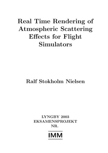
Figure 3: Ewald construction illustrating how Bragg scattering conditions are maintained duringan azimuthal scan.5.1.3 Four-circle diffractometryFor single-crystal experiments with monochromatic radiation, it is quite apparent that one shouldstrive to maintain the maximum flexibility in orienting the crystal. One way to accomplish this isto mount the crystal in an Eulerian cradle, as illustrated in fig. 4 (note the alternative nomenclature for the angles). The whole assembly, including the detector arm, is known as a four-circlediffractometer. With a four-circle diffractometer, one can in principle (barring mechanical collisions and shadowing effects) access all nodes of the reciprocal space that are accessible for agiven wavelengh. It is an easy exercise in the Ewald construction (left to the reader) to showthat the accessible nodes are contained within a sphere of radius 4π/λ, centered on the origin ofreciprocal space. This is equivalent to saying that the shortest accessible d-spacing is 1/2 thewavelength — a statement that can be easily verified from Bragg law by setting θ to have itsmaximum value (90 in backscattering; the λ/2 limit is often referred to as the Bragg cut-off).Modern four-circle diffractometers often employ an alternative, more open geometry, known asκ geometry; here the κ-axis, which replaces the χ-axis, is not perpendicular to the Ω-axis, butforms an angle of approximately 60 with it.13

Figure 4: The geometry of a “four circle” single-crystal diffractometer. The “four circles” (actually four axes) are marked “φ”, “χ”, “Ω” and “2θ”. The 2θ and Ω angles are also known as γ andη — a notation we will often employ in the remainder to avoid clutter and confusion with othersymbols (e.g., the solid angle)5.2 Powder diffraction5.2.1 Debye-Scherrer conesA “powder” sample is a more or less “random” collection of small single crystals, known as“crystallites”. As explained more thoroughly in Appendix III, the cross section for the wholepowder sample depends on the modulus of the scattering vector q but not on its direction.For a monochromatic incident beam, the 2θ angle between the incident and scattered beam isfixed for a given Bragg reflection, but, as we just said, the angle around the incident beam isarbitrary. It is easy to understand that the locus of all the possible scattered beams is a conearound the direction of the incident beam.For monochromatic powder diffraction, the scattered beams form a series of cones(fig. 5), known as Debye-Scherrer cones (D-S cones in the remainder), one for each“non-degenerate” (see below) node of the reciprocal lattice.It follows naturally that all the symmetry-equivalent RL nodes, having the same q, contribute to the same D-S cone. This is also illustrated by the Ewald construction in fig. 6.Moreover, accidentally degenerate reflections, having the same q but unrelated hkl’s, alsocontribute to the same D-S cone. This is the case for example, for reflections [333] and[115] in the cubic system, since 32 32 32 12 12 52 .14

Figure 5: Debye-Scherrer cones and the orientations of the sets of Bragg planes generating them.5.2.2 The Debye-Scherrer geometryThe Debye-Scherrer geometry employs a parallel beam, and the sample has a roughly cylindirical symmetry. The sample is contained in a tube (neutrons) or capillary (x-rays), and is uniformlyilluminated by the incident beam. The detector(s) are placed on a ”detection cylinder” (fig. 7,generally covering only a small portion of the cylinder, near the scattering plane. The typical set-up used for laboratory x-ray diffraction employs a single detector, and a series of slits(often of the multi-lamellar type, known as “Soller slits”) to define the incident and scatteredbeam directions. The main advantage of this geometry is that it is easy to rotate the samplearound its axis, thereby obtaining a good powder average and eliminating at least part of the nonrandomness of the real powder sample (preferred orientation). Also, geometrical aberrations onthe Bragg peak positions can be reduced or eliminated by employing Soller slits. Therefore, theDebye-Scherrer geometry is generally employed to obtain quantitative intensity measurements.Another advantage of this geometry is that it is easy to use many detectors simultaneously, as itis done in reactor-based neutron diffractometers, such as D20 and D2B at the ILL (see feig. 7.There are several variants of the Debye-Scherrer geometry, differing mainly for the degree andtype of collimation, the type of monochromator and the detector technology. An important classof instruments, for both x-rays and neutrons, employs a linear position-sensitive detector (PSD)without scattered-beam collimation. This results in a very large increase of count rates, at theexpense of introducing some aberrations. Another important variant is the analyser geometry,15

Figure 6: Ewald construction for powder diffraction, to represent the crystal being rotated randomly around the direction of the incident beam (the figure actually shows the opposite, forclarity).where the Soller slits on the scattered beam are replaced with an analyser crystal. This results ina considerable intensity loss, but with a much-enhanced resolution and precision. The analysergeometry is frequently employed at synchrotron sources, coupled with a parallel incident beam.Fig. 8 shows a comparative example of X-ray and neutron high-resolution data collected on thesame compound using variants of the the Debye-Scherrer geometry.Figure 7: The Debye-Scherrer powder diffraction geometry, as implemented on a film camera(A) and on a modern constant-wavelength powder diffractometer (B). Note that, in the latter, thefilm has been replaced with an array of 3 He gas tubes.16

Key points to retain about powder diffraction In powder diffraction methods, the intensity around the D-S cones is always integrated,yielding a 1-dimensional pattern. Powder diffraction peaks are usually well-separated at low q, but become increasinglycrowded at high q often becoming completely overlapped. This substantially reducethe amount of information available to solve or refine the structure precisely (seebelow).6Profiles and integrated intensitiesIn all the techniques mentioned in the previous sections, one measured either a certain number of“counts” in the detector (“counting” detectors) or a continuous variable (e.g., the “blackening”of a photographic film, the amount of charge stored in a Charge-Coupled Device (CCD) or in animage plate, etc). Provided that the detector is well designed, it is possible to recover this valuequantitatively and employ it to learn something about the crystal structure (see below). As wehave seen in the previous example, the detected intensity comes in the form of spots, rings or1-dimensional peaks, depending on the technique one employs. With linear position-sensitivedetectors or area detectors, the scattered intensity is in general distributed among more than one“pixel” or “bin”.When dealing with diffraction data from crystalline matter, one is in general left with twochoices: Sum up the pixels or bins pertaining to a single node of the RL, obtaining the so-calledintegrated intensity. This is the method of choice for single-crystal diffraction. As onecan perhaps guess from eq. 10, the integrated intensity is proportional to the squaredmodulus of the structur factor, but with some important geometrical factors. Retain the separate pixels and analyse the profile of the peaks. This is the method ofchoice for powder diffraction, where peak overlap prevents unambiguous assignmentof the intensity to a single RL node. In this case, single-node integrated intensitiesare extracted as part of the analysis.In either case, an essential step in the quantitative analysis of diffraction data is to calculateintegrated intensities from the expression of the cross section (eq. 10).The calculation is slightly different for different experimental geometries, but in all cases italways involves converting the 3-dimensional δ- function in eq. 10 into appropriate polar17

Figure 8: X-ray and neutron high-resolution powder diffraction at a glance. A: neutron powderdiffraction (D2B-ILL, Grenoble, France, λ 1.594) and B synchrotron x-ray diffraction (X7aNSLS, Brookhaven, USA, λ 0.5000) data on the pyrochlore compound Tl2 Mn2 O2 . Bothinstruments employ variants of the Debye-Scherrer geometry. Note how the intensity decays athigh q much more for the X-ray data, due to the X-ray form factor. The structure is cubic, andpeak overlap is minimal for the neutron data, but it is clearly visible at high q for the X-ray data,collected with a much shorter wavelength. Both data sets are fitted using the Rietveld method(see below)coordinates, followed by integration over some of the variables. Calculations for differentexperimental geometries are provided in Appendix III.18

The key point to remember are the following The integrated intensity can always be reduced to a dimensionless quantity (counts). The general expression for the integrated intensity (number of particles) isPτ Nc d3v0 mτ F (τ ) 2 P(γ)L(γ)Aτ (λ, γ)Finc(25)where- Nc is the number of unit cells in the sample.- d is the d-spacing of the reflection.- v0 is the unit-cell volume.- mτ (powder diffraction only) is the number of symmetry-equivalent reflections. Thisaccounts for the fact that in powder diffraction these reflections are not separable, and will always contribute to the same Bragg powder peak (see previousdiscussion and fig. 6.- P(γ) is the polarisation factor (dimensionless), which we have already introduced.- L(γ) is the so-called Lorentz factor (dimensionless), and contains all theexperiment-specific geometrical factors arising from the δ-function integration.- Aτ (λ, γ) (dimensionless) is the attenuation and extinction coefficient, whic

lecture will be devoted to the discussion of crystal defects, starting from the ones arising from the finite size of real crystals. 2 Cross section for a “small” perfect single crystal Our goal in this section is to calculate the scattering cros