WIXLIB

16LIST OF FIGURESAlso thank to my sister Susanne Stokholm Nielsen for grammatical revision.Finally a big thank to my girlfriend Charlotte Højer Nielsen for her support,encouragement and for putting up with me throughout the project.Technical University of Denmark DTUSeptember 2003Ralf Stokholm Nielsen

17Chapter 1IntroductionIn the past, real time rendering of outdoor scenes in flight simulator applications has primarily dealt with the problem of increasing the geometricdetail of the part of the terrain visible to the user.During the last five years of the 20’th century, advances in consumer graphics hardware have enabled amazing improvements in the raster capabilitiesof pc’s. With the change of the millennia, consumer graphics hardwarecapable of transforming and lighting vertices began appearing. This has,over a few years, lead to graphics processors GPU’s that are becoming increasingly flexible and capable of performing small programs, both on thepixel and vertex level.The adversity and raw processing power of modern GPU’s are currentlyshifting the focus of real time rendering towards some of the areas traditionally associated with (non real time) image synthesis. This has openedthe opportunity for rendering much more realistic images.Realism can in this context be interpreted as either physical realism, meaning that the rendering systems use models that closely resemble the physicsof lights interaction with the environment, or visual realism, meaning thatthe generated images display a convincing similarity with the real world.In the following, realism will, unless explicitly stated, refer to the latterdefinition.

181.1Chapter 1. IntroductionBackgroundFlight simulators have always represented an area where the separationbetween professional software and ”games” has been blurry. Producers ofPC flight simulators have competed to supply the most realistic simulationof the flight dynamics and avionics of the aircraft. The focus on realism hasalso meant that simulators are presented with a challenge when it comesto rivaling this realism in the rendering of the environment.The rendering of the environment in a flight simulator lacks many of theshortcuts present in other games. A flight in a flight simulator spans apotential long time period and a vast area. In addition, flight simulatorsare often set in a known environment, requiring the landscape to be recognizable. The time covered prohibits the use of static coloring of the sky andlandscape, the free nature of flight prohibits the use of a textured skydometo display cloud effects, and the large area covered during flight requiresthe processing of enormous amounts of data in order to render the terrain.Although algorithms for rendering huge terrain datasets have been available for some time now [15, 11, 5], there are still plenty of areas that canbe improved tremendously. Recent works have begun investigating theuse of modern shader technology for simulating atmospheric scattering effects [10, 3], while others are investigating the use of similar technologiesto transfer techniques such as HDR (High Dynamic Range) imagery torealtime applications [6, 7].Even though the processing power has increased enormously since the firstflight simulators were designed, it is still unrealistic to imagine a physicallybased rendering system, calculating the radiative transfer throughout thescene. Consequently, the rendering system still needs to be designed toimitate realism rather than to be realistic.Two different approaches exist for rendering atmospheric scattering effectsin real time. Dobashi proposed a volumetric rendering method capable ofcapturing things like shafts of light and shadows cast by mountains [3].Hoffman and Preetham proposed a simpler approach where atmosphericscattering is calculated at the individual objects based on distance fromthe viewpoint and angle to the sun, the system was implemented usingvertex shaders. Both methods have advantages and disadvantages, andnone of them can directly fulfil the requirements for implementation in aPC flight simulator.

1.21.2Problem19ProblemThe purpose of this work is to develop a system of shades to simulate theeffects of atmospheric scattering in a flight simulator environment. Theproblem is divided into two sub problems; rendering of the sky and rendering of the landscape.For the sky, the system must be capable of capturing the change in colorwhen the sun travels over the skydome during the day. It must also becapable of capturing the change in color that results when the observerchanges altitude. Both effects are important to the sensation of immersion.For the terrain, the purpose is to create a system capable of simulating theeffects of areal perspective, the effect of observing a distant object throughthe atmosphere, see section 2.5. The system must be able to simulate thechange in color of distant objects. It must also be capable of simulatingthe change in visibility for different view angles compared to the directionof the sun. Last, it must be capable of capturing the change in arealperspective when changing observer altitude. Areal perspective is centralfor the human ability to determine distance and, as a result, plays a centralrole to the realism of a flight simulator rendering system.Both areal perspective and sky color change with the altitude of the sunabove the horizon and with the amount of aerosols in the atmosphere. Thesystem has to be able to cope with these changes fluently.Flight simulators are some of the most processor intensive real time rendering systems and, consequently, the developed system must be able towork at real time rates while leaving recourses for other tasks like flightmodelling, AI, avionics etc.1.3LimitationsThe main focus of this work is on creating a system suitable for inclusionin a flight simulator. The aim is to be able to convincingly recreate theeffects of atmospheric scattering on a subjective level.The physics of atmospheric scattering are crucial to understanding theproblem but the physical accuracy of the system is irrelevant. It is notintended to accurately simulate a given physical environment but to present

20Chapter 1. Introductionthe virtual pilot with some of the phenomenons he would expect to observein the real world.To demonstrate the system, a small application capable of rendering aheight field and a skydome is developed. These are developed to demonstrate the shaders and they will not be highly optimized.The system is targeted at PC systems equipped with a recent graphics card.1.4OutlineIn chapter two, the theory of atmospheric scattering is presented. It isa rough overview of the system, intended to provide the reader with abasic understanding of the theory required for understanding the proposedsimplifications.Chapter three explains the basic problem of rendering scattering effects andoutlines the work of previous researchers in the area of rendering scatteringeffects.In chapter four, the technology behind modern rendering hardware andAPIs is described to provide the reader with a basic understanding of thetechnology, required for the understanding of the proposed implementation.In chapter five, the hypothesis is developed, based on the work of previousresearchers and the theory described in chapter two.Chapter six describes the implementation of the rendering system proposedin the hypothesis.In chapter seven, the renderings produced by the implemented system areshown.Chapter eight discusses the results and provides ideas for improvementsand future development.Chapter nine presents the conclusion and is followed by appendices.

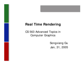
21Chapter 2Atmospheric ScatteringAs sunlight penetrates the atmosphere it may be absorbed, scattered, reflected or refracted before reaching the surface. Humans perceive light withthe help of antenna-like nerve endings located in our eyes (rods and cones).Our eyes detect different intensities (light and dark) and different colorsdepending on the wavelengths of visible radiation.White light is a combination of all wavelengths from 400 700 nm in nearlyequal intensities. The sun radiates almost half of its energy as visible light.The peak intensity of the sun’s electromagnetic radiation corresponds tothe color yellow. Because all visible wavelengths from the sun reach thecones in nearly equal intensities when the sun is close to zenith (with aslight peak at yellow), the sun appears yellowish-white during the middleof the day.The attenuation of light in the atmosphere is caused by absorbtion andscattering, and can be divided into effects that remove and add light toa given viewing ray. Absorbtion of visible light is negligible except forabsorbtion in the ozone layer [8]. As a result, the atmosphere below theozone layer can be treated as a scattering media only. Scattering is a resultof the interaction between the electromagnetic field of the incoming lightwith the electric field of the atmospheric molecules and aerosols [16]. Thisinteraction is synchronized and, as a result, the scattered light has thesame frequency and wavelength as the incoming light. Scattering differswith particle size and varies with wavelength. For this reason, the spectralcomposition of the scattered light differs from that of the incoming light.

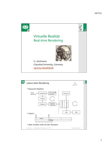
22Chapter 2. Atmospheric ScatteringSunlightPaPss : Sunlight PathAtmosphereP: Scattering Pointθ: Scattering Anglehs: Scattering altitudeh: Observer Altitudes:Multiple ScatteringViewing PathPv: Observation PointEarthFigure 2.1: The sizes and parameters involved in a single scattering event inthe atmosphere.Figure 2.1 demonstrates a single scattering event. At a point P light fromthe sun is scattered into the viewing path (single scattering). Light alreadyscattered one or more times also arrives and is scattered at P (multiplescattering). The angle between the viewing path and the direction of thesunlight θ is called the scattering angle. This angle is the independent variable in the scattering phase function described later in the sections on Mieand Rayleigh scattering. The total amount of light arriving at the viewpoint Pv is the combined effect of scattering effects along the entire viewingpath s. The light incident on the viewdata from the single scattering eventat P is attenuated by scattering before reaching the viewpoint Pv .Atmospheric scattering will both add and remove light from a viewing ray.This is the effect that causes the brightening of distant dark object alongwith a loss of contrast (see figure 2.2). This effect is very important to thehuman ability to assess distances even at surprisingly short ranges [17].Any type of electromagnetic wave propagating through the atmosphere is

23Figure 2.2: The extinction of the mountains far from the viewpoint caused byatmospheric scattering.affected by scattering. The amount of scattered energy depends stronglyon the ratio of particle size to the wavelength of the incident wave. Whenscatterers are small relative to the wavelength of incident radiation (r λ/10), the scattered intensity on both forward and backward directions isthe same. This type of scattering is referred to as Rayleigh scattering. Forlarger particles (r λ/10), the angular distribution of scattered intensitybecomes more complex with more energy scattered in the forward direction.This type of scattering is described by Mie scattering theory.When the scattering particles are considered to be isotropic, the shape ofthe scattering phase function is uniform with respect to the direction of theincoming beam. This is not always the case for atmospheric particles, butany error introduced by making the assumption that they are, is evened outby the large number of randomly oriented particles [16] and, consequentlyfor this thesis, particles are considered isotropic.When the relative distance between the scattering particles is large compared to the particle size, the scattering pattern of each function is unaf-

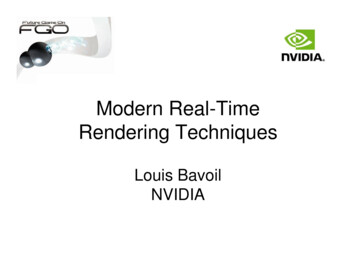
24Chapter 2. Atmospheric Scatteringfected by the presence of other particles. This is the case in the atmosphereand, as a result, the scattering from a path in the the atmosphere can be approximated, using a single function for each of the two types of scattering;scattering by particles and scattering by molecules [16].A small fraction of the scattered light is scattered again one or more timesbefore leaving the scattering media. This is referred to as multiple scattering. In most situations, the effects of multiple scattering on the intensity ofthe direct beam are barely noticeable. This is the case for scattering in theatmosphere on a clear day [16, 17]. However, ignoring multiple scatteringwhen trying to describe the color of clouds will create noticeable artifacts[9]. In general, multiple scattering influences are more significant in turbidor polluted atmospheres.2.1Rayleigh ScatteringRayleigh scattering refers to the model of atmospheric scattering causedby molecules (clean air). In this context, only scattering of visible lightis relevant. The volume angular scattering coefficient, or phase functionβ λ (θ), describes the amount of light at a given wavelength λ scattered ina given direction θ. For Rayleigh scattering, this is given by [13]. 2 π 2 n2 1 1 cos2 θ(2.1)β(θ) 42N λwhere θ is the angle between the view angle and the sun direction, n isthe refractive index of air, N is the molecular density and λ the wavelength of light. The important property of the Rayleigh scattering phasefunction (2.1) is the λ14 dependency of wave length. The net result of thisproperty is that shorter wavelengths are scattered much more than longerwavelengths, approximately an order of magnitude for the visible spectrum(400 700nm). This is the main reason why the sky is blue.The total Rayleigh scattering coefficient βR can be derived from equation(2.1) by integrating over the total solid angle 4π 2Z 4π8π 3 n2 1(2.2)βR β(θ)dΩ 3N λ40The total scattering coefficient describes the total amount of light removedfrom a light beam by scattering.

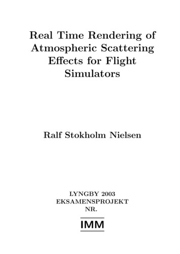
2.2Mie 00.511.522.5-0.5-1-1.5Figure 2.3: Rayleigh phase function, the intensity of light scattered into theviewing path, as a function of the angle from the sun.2.2Mie ScatteringMie scattering theory is a general theory applicable to scattering caused byparticles of any size. In this thesis, Mie scattering theory is used exclusivelyfor describing the scattering caused by atmospheric particles (aerosols) withsizes equal to or larger than the wavelength of the scattered light.Rayleigh scattering is a subset of Mie scattering. Consequently, Mie scattering theory will yield the same results as Rayleigh scattering when applied to small particles. If assuming a certain average size of the scatteringparticles, the Mie scattering function can be written as [20].β(θ) 0.434c4π 20.5βM (θ)λ2(2.3)Where c is the concentration factor which varies with turbidity T and isgiven by [20].c (0.6544T 0.6510) · 10 16(2.4)and βM describes the angular dependency (phase function)[20]. βM varieswith the size of the scattering particles and gives the shape of the angular

26Chapter 2. Atmospheric ScatteringFigure 2.4: Mie angular scattering functions. The top left image is identical tothe Rayleigh phase function, demonstrating that Rayleigh scattering theory is aλsubset of Mie scattering for small particles r 10Mie scattering function (figure 2.4). The total Mie scattering factor isdetermined by.4π 2βM 0.434cπ 2 K(2.5)λWhere K varies with λ and are 0.671 .2.2.1Henyey-Greenstein Phase FunctionMie theory is in general far more complicated than Rayleigh theory. However, for the application to real time rendering, the angular scattering func¡ v 22(2.3) and (2.5) are slightly incorrect 4πwhere v is Junge’sshould be 2πλλ2exponent. However a value of 4 is used for the Mie scattering model in this thesis. Thisis taken from [20, 10]1 Both

2.3Optical Depth271.51.5g 0.20SunDirection1g -0.5-0.5-1-1-1.5-1.50.511.522.5(a) Shape of the HG phase function for (b) Shape of the HG phase function forg 0.55g 0.20Figure 2.5: The shape of the Henyey-Greenstein phase function with varyingg. The Henyey-Greenstein phase function is a simplification of the general Miescattering phase function as shown in figure 2.4.tion can be approximated using the Henyey-Greenstein phase function [10].ΦHG (Θ) 1 g234π (1 g 2 2cos(θ)) 2(2.6)Where g is the directionality factor. Figure 2.5 shows how the shape of thephase function varies with the value of g.The Henyey-Greenstein (HG) phase function belongs to a class of functionsused primarily for their mathematical simplicity than for their theoreticalaccuracy. The HG function is simply the equation of an ellipse in polarcoordinates centered at one focus. It can be used to simulate scattereingwith the primary scattering is in the backward direction (g 0) or theforward direction (g 0) [2]2.3Optical DepthA term widely used in atmospheric optics is optical depth, which is applicable to any path characterized by an exponential law.

28Chapter 2. Atmospheric ScatteringOptical depth for a given path can be derived as the integral of the scattering coefficient of all subelements ds of the given path.Zβ(s)ds(2.7)T SWhere β(s) is the scattering coefficient (combined Mie and Rayleigh totalscattering coefficients) that varies from day to day and with altitude.Optical depth can be used directly to calculate the attenuation over apath. Given an incident spectral distribution I0 , the attenuated spectraldistribution I arriving at the observer after passing the atmosphere withthe optical depth T is given by.I I0 · e T(2.8)Optical depth is a measure of the amount of atmosphere penetrated alonga given path. This means that optical depth is a result of the length of thepath and the average atmospheric density along the path.Optical depth can be separated into the molecular (Rayleigh) and aerosol(Mie) optical depths.2.4Sky ColorThe color of the clear sky has always amazed people. The blue color of thesky is a result of inscattering of light from the sun.

The thesis is related to the areas of computer graphics, real time rendering and atmospheric scattering. The reader is expected to be familiar with engi-neering mathematics and the fundamental principles of computer graphics and real time rendering. Acknowledgements I take this oppo