WIXLIB

4CHAPTER 1. CROSS-SECTIONSalong the beam. But now that the particles are scattering out from a pointliketarget, the actual count through an area falls off with the inverse of the distancesquared. But we are now measuring with angles, so we want the count througha solid angle.[Eventually I’ll add figures to help illustrate this.]Experimentally, what we measure as the physically meaningful quantity israte of outgoing particles through a solid angleoverrate of incoming particles through an areaThis ratio has units of area, and we call it the cross-section. As befits theorigin story of scattering, with Geiger and Marsden trading turns staring at alittle patch of phosphorescent screen, it has become our window on the submicroscopic world.Also befitting the origins of scattering is the main unit of cross-sections.Historically, in the century after Newton’s invention of calculus mathematicalphysics was largely taken over by French mathematicians, hence the preponderance of French names: Laguerre, Legendre, and Hermite polynomials are thedaily diet of junior physicists struggling to solve differential equations. Quantummechanics was dominated by German physicists, hence eigenstates and Ansätze.But in the years between the world wars, English-speaking experimental physicists, began, if not to dominate, then to make significant contributions, and inthe U.S. in particular these often came from rural or working-class backgrounds.Hence the colloquial origin of a term probably as puzzling to non-English speakers as “plum pudding” is to anyone outside the British Commonwealth: the barn,as in the phase, couldn’t hit the broad side of a barn. A barn is 10 24 cm2 .1.1Adding quantum mechanics: current, flux,and the scattering amplitudeI’ve introduced a fundamental idea, which is that we learn about a tiny objectby measuring the ratio of particles out to particles in, and that this ratio hasunits of area and is called the cross section. Now we want to start to developa theory of this scattering, and because the target is very, very tiny, we invokethe theory of tiny things, or, more formally, of tiny action: quantum mechanics.The wave function for incoming particles is easy. We assume a beam ofparticles with uniform momentum p , and in quantum mechanics the momentum An eigenstate of this operator is a planeoperator in coordinate space is h̄i .wave, exp(i p · r/h̄).Normalization of any wave function is crucial in quantum mechanics. WhileI discuss this in detail in section 4.1, for now let’s assume we put our plane wavein a cubic box with each side of length L, so that the volume is L3 . Of course,this ignores the important issue of boundary conditions, so we don’t really have

1.1. THE SCATTERING AMPLITUDE5a true plane wave, but being physicists we set aside that unpleasantness untillater. Then the normalized, sort-of plane wave in a cube L3 is p · r1exp i.(1.1)h̄L3/2Now let’s look at another idea, which is not always emphasized in introductoryquantum texts but which will be fundamental for us: the quantum current. Hereis a brief reminder of the standard motivation: for any time-dependent wavefunction Ψ( r, t), the probability density is of course ρ( r, t) Ψ( r, t) Ψ( r, t).If we do not have a stationary state, that is, if we cannot factorize Ψ( r, t) ψ( r) exp( iEt/h̄)–and although in introductory courses that kind of factorization is often assumed, the most general solutions to the time-dependentSchrödinger equation cannot be so factorized–then ρ( r, t) can change in time.We then invoke an idea from classical fluid flow, that is the continuity equation, ρ( r, t) · J( r, t) 0, t(1.2) r, t) is the current. Most introductory quantum texts show thatwhere J( J h̄ .Ψ Ψ Ψ Ψ2M i(1.3)For a plane wave (1.1) with momentum p , the current isp 1h̄ k 1J plane wave .M VolM Vol(1.4)Here I’ve introduce the wave vector k p /h̄, whose magnitude k is called thewave number, which has dimensions of 1/length; many of our results will bestated in terms of the wave number.Note that the current for a plane wave in a box, (1.4) has exactly units oftime 1 area1 , that is, we can interpret it as a flux. This will be very importantto us later!So much for the incoming particles. What about the outgoing particles? Because the particles are scattered off a target that is, macroscopically, a point, wecan no longer talk about plane waves, but rather spherical waves. An outgoingspherical wave isexp(ikr),(1.5)ra result I’ll later justify using Green’s functions (chapter to be written). Becausewe want/know our final result to depend upon the scattering angle, we furtherwriteexp(ikr)ψout f (θ),(1.6)rwhere f (θ) is the scattering amplitude. Here we have not normalized to a box,or else absorbed it into the definition of f . To find the flux for this outgoing

6CHAPTER 1. CROSS-SECTIONSwave, remember that in spherical coordinates the gradient is êr êθ 1 êφ 1 rr θr sin θ φ(1.7) 1ψout ,r(1.8)so that out ikêr ψout O ψand as r only the first term survives. Then the current for ψout ish̄k êr f (θ) 2 .J out r M r 2(1.9)When this scatters at an angle θ the amount of flux through a solid angle Ωat a distance r, and thus through an area Ωr2 , ish̄k f (θ) 2 Ω.MNow let’s put these together. Dropping the normalization to a box of volume L3 , we consider the full scattering wavefunction, with both incoming andoutgoing pieces, Ψscatt . We can only “measure” the wave function at a “large”distance r from the target, which means Ψscatter eik· r f (θ)r exp(ikr).r(1.10)The cross section is just the ratio, of the incoming and outgoing, that is,dσ f (θ) 2 .dθ(1.11)Hence, in much of what we will do in this book is to find ways to characterizeand numerically calculate the scattering amplitude f , and thus the cross-sectionσ, through concepts such as phase shifts, the S-matrix, and others.1.2Other matters, maybeIncluding a brief discussion of the Born approximation, Rutherford scattering,and form factors.1.3Project 1At the end of each chapter I will propose for you a project to help you pulltogether your knowledge and skills.For this chapter, I want you to hunt down experimental cross-sections inyour field. Despite its heavy reliance upon theory and rigorous mathematics,like all science physics is ultimately and always empirical, and the best wayto become skilled in the topic is to have a store of knowledge of experimentalresults.

Chapter 2Phase shifts and the partialwave decompositionOne way to characterize or parameterize cross-sections σ or the scattering amplitude f (θ), which I introduced in the first chapter, is through phase shifts.Phase shifts start with the idea that, far away from the interaction region, thatis, where the projectile interacts with the target or, more formally, where theinteraction potential vanishes, the particle is free. For particles with zero relative angular momentum, that is, with orbital angular momentum 0 (alsocalled an s-wave), this looks like some combination of sines and cosines, thatis, simple waves. As discussed in the next section, if there were no scatteringpotential, the solution would be a pure sine wave everywhere. If we add a scattering potential, however, beyond the range of the potential the particle is stillfree, but the phase of the wavefunction is now shifted: hence the name.Most texts derive phase shifts from the so-called partial wave decompositionor expansion, where one takes solutions to the Schrödinger equation and decompose it into part of good orbital angular momentum. We will do so belowin section 2.3, but we will first simply explore the idea of a phase shift beforecarrying out this somewhat complicated derivation.2.1What is a phase shift?The basic idea is that scattering is localized, so that at some distance the scattering particle is free. The radial Schrödinger equation a particle of mass mcish̄2 d2h̄2 ( 1)u(r) u(r) V (r)u(r) Eu(r)(2.1) 2m dr22mr2where is the orbital angular momentum. First, let’s think about the case with 0, that is, s-wave scattering. For a free particle, V 0, the solutions are7

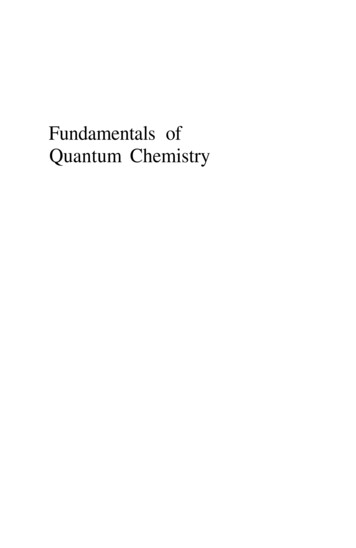
8CHAPTER 2. PHASE SHIFTS2"free" particleshifted free particleu(r)10-1-20510r15Figure 2.1: Illustration of the shift in s-wave ( 0) wave function due to a hardsphere at r 2 (dashed red vertical line). Solid black line is the “free” particlewave function, while the blue dotted line is for the particle in the presence ofthe hard sphere.linear combinations of sine and cosine functions, that is,u(r) A sin(kr) B cos(kr),(2.2) where k p/h̄ 2mE/h̄ is the wavenumber. Now if the potential vanisheseverywhere, the only boundary condition is at the origin and u(0) 0 and weare restricted to sine functions, that is, B 0.But now suppose V (r) 6 0 for r within some radial distance R. For r 0we stil have a free particle, but we no longer have the boundary condition.Therefore we can have B 6 0. More generally we writeu(r) C sin(kr δ),(2.3)where by trigonometric identities A C cos δ, B C sin δ, and finally tan δ B/A. We’ll see later that the phase shift δ is a function of the wavenumber k,which mean it depends upon the momentum p or the energy E.Example: the hard sphere. As a simple example, consider the hardsphere, where V for r R. This means we have a boundary conditionu(R) 0 or sin(kR δ) 0; hence δ(k) kR. This is shown in Fig. 2.1 for aparticle with orbtial angular momentum 0 (or s-wave). The “free” particleis just a sine function, with the boundary condition u(0) 0, here seen as theblack solid line. The blue dotted line shows the shift in the free particle wave

2.2. SCATTERING OFF A FINITE SQUARE WELL POTENTIAL9function, which now has a boundary condition at u(R) 0. In this exampleR 2. This is a key example of phase shifts, and all other cases are just morecomplicated cases of this.What about for 0? Then the free particle solutions are spherical Besseland spherical Neumann functions:u (r) A rj (kr) B rn (kr).(2.4)The basic properties of spherical Bessel functions, including how to numericallygenerate them, can be found in section C.1 of the appendices. For now, justknow that sin x π2,(2.5)j (x) x x cos x π2.(2.6)n (x) x xThe minus sign in front of the limit of the spherical Neumann function explainsthe difference in sign between (2.4) and (2.2). From this we can generalize phaseshifts for any value of : πu (r) rj kr δ (k) ,(2.7)2wheretan δ B .A (2.8)Example: the hard sphere redux Consider again the hard sphere butfor arbitrary . We have the boundary conditionu (R) A Rj (kR) B Rn (kR) 0,ortan δ (k) 2.2B j (kR) .A n (kR)(2.9)(2.10)Scattering off a finite square well potentialWe will be using the finite square well of depth V0 and radius R, that is, V0 , r R,V (r) (2.11)0, r Rover and over; we will solve it analytically, but then use it as a test case fornumerical calculations.First, let’s do it for s-wave scattering, or 0. This is easier to visualize.To solve the finite square well, we divide and conquer two regions: region 1 isfor 0 r R, and region 2 is for R r ; the radial wavefunctions u1,2 (r)

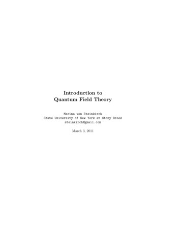
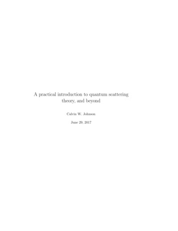
10CHAPTER 2. PHASE SHIFTSand their first derivatives must match at r R. In both cases the solutions aresine functions; in region 1, with a boundary condition u1 (0) 0, it isu1 (r) A sin Kr,where E h̄2 K 2 /2m V0 , that is,p2m(E V0 )K h̄and in region 2, we can either take sine and cosine functions, or, more directly,a sine function with a shift phase:u2 (r) sin(kr δ), where k 2mE/h̄. You will note I did not put a normalization constant onu2 . For now we only need the relative normalization between u1 and u2 ; theabsolute normalization for scattering states we put off until section 4.1.To find the phase shift δ, we need to match at r R both the wavefunctions,u1 (R) u2 (R),A sin KR sin(kR δ),(2.12)and their first derivatives, u01 (R) u02 (R),AK cos KR k cos(kR δ).(2.13)Finally we divide (2.12) by (2.13) to eliminate the constant A and getk tan KR K tan(kR δ).Solving, we find ktan KR(2.14)K We can simplify this a bit by introducing K0 2mV0 /h̄, so that K pK02 k 2 . We’ll use this later.Fig. 2.2 shows the 0 phase shift for a square well with m h̄ 1 andfor a radius R 1, for various depths V0 . Note that at V0 1 the phase shiftrises sharply, while at V0 1 it starts off negative. As we’ll discuss later, whathas happens is as V0 increases, a bound state appears.The apparent discontinuity in the phase shift for V0 1.5 is really justan ambiguity in angle: here δ is restricted to be between π and π radians.Because of this ambiguity, it is sometimes convenient to plot k cot δ0 , shows inFig.2.3 . Shortly we will see that we can interpret the y-intercept and slopeof k cot δ in terms of fundamental quantities called the scattering length andeffective range. Again, as the y-intercept passes through zero, we will see thiscorresponds to a bound state.Notice in Fig. 2.2 that as one increases V0 , the phase shift is initially positive,but with increasing slope. As one goes from V0 1 to V0 1.5, however theδ kR tan 1

2.2. SCATTERING OFF A FINITE SQUARE WELL POTENTIAL111.51δ0 (rad)0.50V0 0.25V0 0.5V0 1.0V0 1.5-0.5-1-1.500.20.40.60.81EnergyFigure 2.2: 0 phase shift δ0 (in radians) for a square well with m h̄ R 1 for several depths V0 , versus energy h̄2 k 2 /2m.V0 0.25V0 0.5V0 1.0V0 1.5k cot δ0642000.20.40.60.81EnergyFigure 2.3: k cot δ0 for a square well with m h̄ R 1 for several depths V0 ,versus energy h̄2 k 2 /2m.

12CHAPTER 2. PHASE SHIFTSphase shift become negative. At the same time one sees the y-intercept inFig. 2.3 pass through zero from positive to negative. Later, when we discussLevinson’s theorem, we will see both of these are associated with a new boundstate appearing as V0 is increased (also see Fig. 4.2).Exercise 2.1: Using any numerical platform you like (Python, MatLab, Mathematica, C/C , Fortran.) reproduce Figs. 2.2 and 2.3. Go futher and increasethe depth. Does the y-intercept of k cot δ0 become positive again?Exercise 2.2: Square well with a hard core. Consider a potential with a hardcore out to some Rc , and an attractive square well of depth V0 from Rc r R.Find the 0 phase shifts analytically.We can also generalize to angular momenta with 0, where the general‘free particle’ solution is (2.4). For u1 (r), we have the boundary conditionu1 (0) 0, which only the spherical bessel function j satisfies:u1 (r) rj (Kr)(2.15)while for r R we have the general solutionu2 (r) A rj (kr) B rn (kr).(2.16)Again we match the wavefunctions at the boundary,Rj (KR) A Rj (kR) B Rn (kR).The overall factor of R of course cancels out. We also need to match derivativesacross the boundary. For that we need (C.8), e.g., d 1d(rj (kr)) (krj (kr)) k rj 1 (kr) rj (kr)drd(kr)krand similarly for the Neumann function, and after cancelling R from both sides,obtain 1K j 1 (KR) j (KR)KR 1 1 k A j 1 (kR) j (kR) B n 1 (kR) n (kR)kRkRTo get the phase shift, we need (2.8), let’s first solve for B :B (A j (kR) j (KR))/n (kR)so thattan δ B j (kR)j (KR) 1 .A n (kR)n (kR) A (2.17)

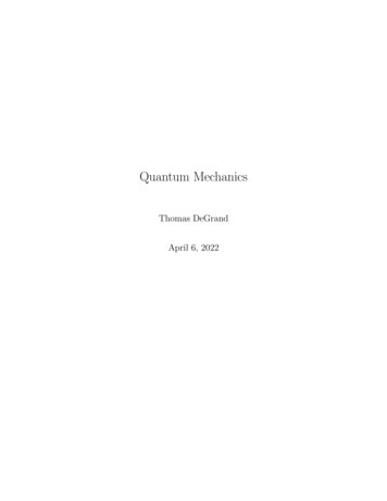
2.2. SCATTERING OFF A FINITE SQUARE WELL POTENTIAL131.51δl (rad)0.50l 0l 1l 2l 3l 4-0.5-1-1.50246EnergyFigure 2.4: Phase shift δ (in radians) for a square well with m h̄ R 1,well depth V0 5, versus energy h̄2 k 2 /2m, for different angular momentum .The dotted red line at δ 0 is to guide the eye.and then 1 1K j 1 (KR) j (KR) k A j 1 (kR) j (kR)KRkR (A j (kR) j (KR)) 1 n 1 (kR) n (kR)n (kR)kRNow, with some algebra, we can solve for A and finally we get the phaseshift,tan δ kj (KR)j 1 (kR) Kj (kR)j 1 (KR)kj (KR)n 1 (kR) Kn (kR)j 1 (KR)(2.18)This can be tested by checking the case 0, withsin xsin x x cos x, j1 (x) xx2cos xcos x x sin xn0 (x) , n1 (x) xx2j0 (x) and indeed it reduces to the correct answer,tan δ0 k tan KR K tan kR.K k tan kR tan KR(2.19)

14CHAPTER 2. PHASE SHIFTSTo see how the phase shifts vary with , see Fig. 2.4. Notice as increases, thephase shifts decrease. This makes sense, because scattering at higher angularmomentum is of necessity more peripheral, and hence, the effect of the potentialis lessened. The phase shifts for 0, 1 start off negative because they bothhave one bound state, while 2, 3, . . . do not have bound states.Exercise 2.3. Confirm for yourself Eqn. (2.18) and that for 0 we regain(2.19).2.3Phase shifts and cross-sections: formal derivationNow that we have some examples of phase shifts, we ask: how do phase shiftsaffect the cross-section? Here’s the short answer: We’ve decomposed the wavefunction into pieces with good angular momentum , the so-called partial waves.In the absence of a scattering potential, the sum all the partial waves for theprojectile is a plane wave. In the presence of a scattering potential, each partialwave undergoes a shift in phase, which in turn causes an interference patternwhich causes the probability to depend upon the angle–the cross-section. Therest of this section works out these relations in depth. This is the starting pointfor many introductory texts, so it’s possible you have seen this before.First, let’s start with the incoming plane wave, and assume that the momentum p and the wave vector k are both in the z-direction. Then the plane waveisexp(i k · r) exp(ikz) exp(ikr cos θ),(2.20)where in the last step I’ve moved into spherical coordinates. We can expandany function in spherical coordinates into spherical harmonics, that is,exp(ikr cos θ) Xg ,m (r)Y ,m (θ, φ);(2.21) ,mexcept we know there is no φ-dependence, so we only need m 0, and Y ,m (θ, φ) P (cos θ) the Legendre polynomial (up to some constant), and soexp(ikr cos θ) Xg (r)P (θ).(2.22) As discussed in the last section, however, we also know that the solutions tothe free Schrödinger equation for angular momentum are spherical Bessel andspherical Neumann functions, and that only the former is regular at the origin.Hence we must haveXexp(ikr cos θ) c j (kr)P (θ).(2.23)

2.3. FORMAL DERIVATION15With some more analysis, one can finally arrive atexp(ikr cos θ) Xi

3 Introducing the S-matrix 24 . While scattering theory is a common topics, I chose to write this book be-cause most quantum mechanics texts give only a brief introduction, and most books on scattering theory emph