Transcription
Lecture 34Rayleigh Scattering, MieScattering34.1Rayleigh ScatteringRayleigh scattering is a solution to the scattering of light by small particles. These particlesare assumed to be much smaller than wavelength of light. Then a simple solution can be foundby the method of asymptotic matching. This single scattering solution can be used to explaina number of physical phenomena in nature. For instance, why the sky is blue, the sunset somagnificently beautiful, how birds and insects can navigate without the help of a compass.By the same token, it can also be used to explain why the Vikings, as a seafaring people,could cross the Atlantic Ocean over to Iceland without the help of a magnetic compass.339
340Electromagnetic Field TheoryFigure 34.1: The magnificent beauty of nature can be partly explained by Rayleigh scattering[182, 183].When a ray of light impinges on an object, we model the incident light as a plane electromagnetic wave (see Figure 34.2). Without loss of generality, we can assume that theelectromagnetic wave is polarized in the z direction and propagating in the x direction. Weassume the particle to be a small spherical particle with permittivity εs and radius a. Essentially, the particle sees a constant field as the plane wave impinges on it. In other words, theparticle feels an almost electrostatic field in the incident field.Figure 34.2: Geometry for studying the Rayleigh scattering problem.
Rayleigh Scattering, Mie Scattering34.1.1341Scattering by a Small Spherical ParticleThe incident field polarizes the particle making it look like an electric dipole. Since theincident field is time harmonic, the small electric dipole will oscillate and radiate like aHertzian dipole in the far field. First, we will look at the solution in the vicinity of thescatter, namely, in the near field. Then we will motivate the form of the solution in the farfield of the scatterer. Solving a boundary value problem by looking at the solutions in twodifferent physical regimes, and then matching the solutions together is known as asymptoticmatching.A Hertzian dipole can be approximated by a small current source so thatJ(r) ẑIlδ(r)(34.1.1)In the above, we can let the time-harmonic current I dq/dt jωqIl jωql jωp(34.1.2)where the dipole moment p ql. The vector potential A due to a Hertzian dipole, aftersubstituting (34.1.1), is J(r0 ) jβ r r0 µdr0e4π r r0 VµIl jβre ẑ4πrA(r) (34.1.3)Near FieldFrom prior knowledge, we know that the electric field is given by E jωA Φ. From adimensional analysis, the scalar potential term dominates over the vector potential term inthe near field of the scatterer. Hence, we need to derive the corresponding scalar potential.The scalar potential Φ(r) is obtained from the Lorenz gauge that · A jωµεΦ.Therefore,Φ(r) 1Il 1 jβr ·A ejωµεjωε4π z r(34.1.4)When we are close to the dipole, by assuming that βr 1, we can use a quasi-static approximation about the potential.1 Then 1 jβr 1 r 1z 1e 2 z r z r z r rrr(34.1.5)or after using that z/r cos θ,Φ(r) 1 Thisis the same as ignoring retardation effect.qlcos θ4πεr2(34.1.6)
342Electromagnetic Field TheoryThis dipole induced in the small particle is formed in response to the incident field. Theincident field can be approximated by a constant local static electric field,Einc ẑEi(34.1.7)The corresponding electrostatic potential for the incident field is then2Φinc zEi(34.1.8)so that Einc Φinc ẑEi , as ω 0. The scattered dipole potential from the sphericalparticle in the vicinity of it is given byΦsca Esa3cos θr2(34.1.9)The electrostatic boundary value problem (BVP) has been previously solved and3Es εs εEiεs 2ε(34.1.10)Using (34.1.10) in (34.1.9), and comparing with(34.1.6), one can see that the dipole momentinduced by the incident field is thatp ql 4πεεs ε 3a Eiεs 2ε(34.1.11)Far FieldIn the far field of the Hertzian dipole, we can start withE jωA Φ jωA 1 · Ajωµε(34.1.12)But when we are in the far field, A behaves like a spherical wave which in turn behaveslike a local plane wave if one goes far enough. Therefore, jβ jβr̂. Using thisapproximation in (34.1.12), we arrive at ββE jω A 2 · A jω(A r̂r̂ · A) jω(θ̂Aθ φ̂Aφ )(34.1.13)βwhere we have used r̂ β/β.34.1.2Scattering Cross SectionFrom (34.1.3), we see that Aφ 0 whileAθ 2 It3 Itjωµql jβresin θ4πris not easier to get here from electrodynamics. One needs vector spherical harmonics [184].was one of the homework problems.(34.1.14)
Rayleigh Scattering, Mie Scattering343Consequently, using (34.1.11) for ql, we have in the far field that4 ω 2 µql jβrεs ε a32 Eθ jωAθ esin θ ω µεEi e jβr sin θ4πrεs 2ε rHφ rε1Eθ Eθµη(34.1.15)(34.1.16)pwhere η µ/ε. The time-averaged Poynting vector is given by hSi 1/2 e {E H }.Therefore, the total scattered power isPs 12 π01 4 β2η εs εεs 2ε2πdφEθ Hφ r2 sin θdθ0 2a6 Ei 2 r2r2(34.1.17) π3 sin θdθ 2π(34.1.18)0But ππ2sin θdθ 0 π3(1 cos2 θ)d cos θsin θd cos θ 0 0 1(1 x2 )dx 143(34.1.19)ThereforePs 4π3η εs εεs 2εs 2β 4 a6 Ei 2(34.1.20)The scattering cross section is the effective area of a scatterer such that the total scatteredpower is proportional to the incident power density times the scattering cross section. Assuch it is defined as 2Ps8πa2 εs εΣs 1 (βa)4(34.1.21)23εs 2ε2η Ei In other words,Ps hSinc i ΣsIt is seen that the scattering cross section grows as the fourth power of frequency sinceβ ω/c. The radiated field grows as the second power because it is proportional to theacceleration of the charges on the particle. The higher the frequency, the more the scatteredpower. this mechanism can be used to explain why the sky is blue. It also can be used toexplain why sunset has a brilliant hue of red and orange. The above also explain the brilliantglitter of gold plasmonic nano-particles as discovered by ancient Roman artisans. For gold,4 The ω 2 dependence of the following function implies that the radiated electric field in the far zone isproportional to the acceleration of the charges on the dipole.
344Electromagnetic Field Theorythe medium resembles a plasma, and hence, we can have εs 0, and the denominator can bevery small.Furthermore, since the far field scattered power density of this particle ishSi 1Eθ Hφ sin2 θ2η(34.1.22)the scattering pattern of this small particle is not isotropic. In other words, these dipoles radiate predominantly in the broadside direction but not in their end-fire directions. Therefore,insects and sailors can use this to figure out where the sun is even in a cloudy day. In fact,it is like a rainbow: If the sun is rising or setting in the horizon, there will be a bow acrossthe sky where the scattered field is predominantly linearly polarized.5 Such a “sunstone” isshown in Figure 34.3.Figure 34.3: A sunstone can indicate the polarization of the scattered light. From that, onecan deduce where the sun is located (courtesy of Wikipedia).34.1.3Small Conductive ParticleThe above analysis is for a small dielectric particle. The quasi-static analysis may not bevalid for when the conductivity of the particle becomes very large. For instance, for a perfectelectric conductor immersed in a time varying electromagnetic field, the magnetic field in thelong wavelength limit induces eddy current in PEC sphere. Hence, in addition to an electricdipole component, a PEC sphere has a magnetic dipole component. The scattered field dueto a tiny PEC sphere is a linear superposition of an electric and magnetic dipole components.5 Youcan go through a Gedanken experiment to convince yourself of such.
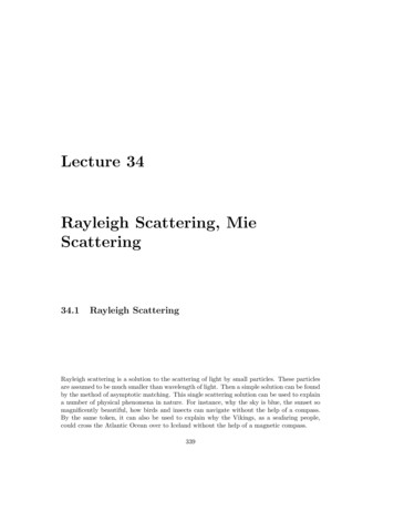
Rayleigh Scattering, Mie Scattering345These two dipolar components have electric fields that cancel precisely at certain observationangle. This gives rise to deep null in the bi-static radar scattering cross-section (RCS)6 of aPEC sphere as illustrated in Figure 34.4.Figure 34.4: RCS (radar scattering cross section) of a small PEC scatterer (courtesy of Shenget al. [185]).34.2Mie ScatteringWhen the size of the dipole becomes larger, quasi-static approximation is insufficient toapproximate the solution. Then one has to solve the boundary value problem in its full gloryusually called the full-wave theory or Mie theory [186, 187]. With this theory, the scatteringcross section does not grow indefinitely with frequency. For a sphere of radius a, the scatteringcross section becomes πa2 in the high-frequency limit. This physical feature of this plot isshown in Figure 34.5, and it also explains why the sky is not purple.6 Scatteringcross section in microwave range is called an RCS due to its prevalent use in radar technology.
346Electromagnetic Field TheoryFigure 34.5: Radar cross section (RCS) calculated using Mie scattering theory [187].34.2.1Optical TheoremBefore we discuss Mie scattering solutions, let us discuss an amazing theorem called theoptical theorem. This theorem says that the scattering cross section of a scatterer dependsonly on the forward scattering power density of the scatterer. In other words, if a plane waveis incident on a scatterer, the scatterer will scatter the incident power in all directions. Butthe total power scattered by the object is only dependent on the forward scattering powerdensity of the object or scatterer. This amazing theorem is called the optical theorem, andthe proof of this is given in J.D. Jackson’s book [42].The true physical reason for this is power orthogonality. Two plane waves can interact orexchange power with each other unless they share the same k or β vector. This happens inorthogonal modes in waveguides [75, 188].The scattering pattern of a scatterer for increasing frequency is shown in Figure 34.6. ForRayleigh scattering where the wavelength is long, the scattered power is distributed isotropically save for the doughnut shape of the radiation pattern, namely, the sin2 (θ) dependence.As the frequency increases, the power is scattered increasingly in the forward direction. Thereason being that for very short wavelength, the scatterer looks like a disc to the incidentwave, casting a shadow in the forward direction. Hence, there has to be scattered field in theforward direction to cancel the incident wave to cast this shadow.
Rayleigh Scattering, Mie Scattering347In a nutshell, the scattering theorem is intuitively obvious for high-frequency scattering.The amazing part about this theorem is that it is true for all frequencies.Figure 34.6: A particle scatters increasingly more in the forward direction as the frequencyincreases.Courtesy of hyperphysics.phy-astr.gsu.edu.34.2.2Mie Scattering by Spherical Harmonic ExpansionsAs mentioned before, as the wavelength becomes shorter, we need to solve the boundaryvalue problem in its full glory without making any approximations. This can be done byusing separation of variables and spherical harmonic expansions that will be discussed in thesection.The Mie scattering solution by a sphere is beyond the scope of this course.7 This problemhave to solved by the separation of variables in spherical coordinates. The separation ofvariables in spherical coordinates is not the only useful for Mie scattering, it is also useful foranalyzing spherical cavity. So we will present the precursor knowledge so that you can readfurther into Mie scattering theory if you need to in the future.34.2.3Separation of Variables in Spherical CoordinatesTo this end, we look at the scalar wave equation ( 2 β 2 )Ψ(r) 0 in spherical coordinates. Alookup table can be used to evaluate · , or divergence of a gradient in spherical coordinates.Hence, the Helmholtz wave equation becomes8 1 2 1 1 22r sin θ β Ψ(r) 0(34.2.1)r2 r r r2 sin θ θ θ r2 sin2 θ φ2Noting the 2 / φ2 derivative, by using separation of variables technique, we assume Ψ(r) tobeΨ(r) F (r, θ)ejmφ(34.2.2)7 But it is treated in J.A. Kong’s book [31] and Chapter 3 of W.C. Chew, Waves and Fields in InhomogeneousMedia [34] and many other textbooks [42, 59, 154].8 By quirk of mathematics, it turns out that the first term on the right-hand side below can be simplified 2 by observing that r12 rr r1 rr.
348whereElectromagnetic Field Theory 2 jmφ φ2 e m2 ejmφ . Then (34.2.1) becomes 1 2 1 m22 βr sinθ F (r, θ) 0r2 r r r2 sin θ θ θ r2 sin2 θ(34.2.3)Again, by using the separation of variables, and letting further thatF (r, θ) bn (βr)Pnm (cos θ)(34.2.4)where we require that dm21 dPnm (cos θ) 0sin θ n(n 1) sin θ dθdθsin2 θ(34.2.5)when Pnm (cos θ) is the associate Legendre polynomial. Note that (34.2.5) is an eigenvalueproblem, and m n .Consequently, bn (kr) satisfies 1 d 2 dn(n 1)2r βbn (βr) 0(34.2.6)r2 dr drr2The above is the spherical Bessel equation where bn (βr) is either the spherical Bessel function(1)jn (βr), spherical Neumann function nn (βr), or the spherical Hankel functions, hn (βr) and(2)hn (βr). The spherical functions are related to the cylindrical functions via [34, 43] 9rπbn (βr) B 1 (βr)(34.2.7)2βr n 2It is customary to define the spherical harmonic ass2n 1 (n m)! mYnm (θ, φ) P (cos θ)ejmφ4π (n m)! n(34.2.8)The above is normalized such that Yn, m (θ, φ) ( 1)m Ynm(θ, φ)and that 2ππsin θdθYn 0 m0 (θ, φ)Ynm (θ, φ) δn0 n δm0 mdφ0(34.2.9)(34.2.10)0These functions are also complete10 if like Fourier series, so that XnX00 Ynm(θ0 , φ0 )Ynm (θ, φ) δ(φ φ )δ(cos θ cos θ )(34.2.11)n 0 m n9 By a quirk of nature, the spherical Bessel functions needed for 3D wave equations are in fact simpler thancylindrical Bessel functions needed for 2D wave equation. One can say that 3D is real, but 2D is surreal.10 In a nutshell, a set of basis functions is complete in a subspace if any function in the same subspace canbe expanded as a sum of these basis functions.
Bibliography[1] J. A. Kong, Theory of electromagnetic waves.New York, Wiley-Interscience, 1975.[2] A. Einstein et al., “On the electrodynamics of moving bodies,” Annalen der Physik,vol. 17, no. 891, p. 50, 1905.[3] P. A. M. Dirac, “The quantum theory of the emission and absorption of radiation,” Proceedings of the Royal Society of London. Series A, Containing Papers of a Mathematicaland Physical Character, vol. 114, no. 767, pp. 243–265, 1927.[4] R. J. Glauber, “Coherent and incoherent states of the radiation field,” Physical Review,vol. 131, no. 6, p. 2766, 1963.[5] C.-N. Yang and R. L. Mills, “Conservation of isotopic spin and isotopic gauge invariance,” Physical review, vol. 96, no. 1, p. 191, 1954.[6] G. t’Hooft, 50 years of Yang-Mills theory.World Scientific, 2005.[7] C. W. Misner, K. S. Thorne, and J. A. Wheeler, Gravitation.Press, 2017.Princeton University[8] F. Teixeira and W. C. Chew, “Differential forms, metrics, and the reflectionless absorption of electromagnetic waves,” Journal of Electromagnetic Waves and Applications,vol. 13, no. 5, pp. 665–686, 1999.[9] W. C. Chew, E. Michielssen, J.-M. Jin, and J. Song, Fast and efficient algorithms incomputational electromagnetics. Artech House, Inc., 2001.[10] A. Volta, “On the electricity excited by the mere contact of conducting substancesof different kinds. in a letter from Mr. Alexander Volta, FRS Professor of NaturalPhilosophy in the University of Pavia, to the Rt. Hon. Sir Joseph Banks, Bart. KBPRS,” Philosophical transactions of the Royal Society of London, no. 90, pp. 403–431, 1800.[11] A.-M. Ampère, Exposé méthodique des phénomènes électro-dynamiques, et des lois deces phénomènes. Bachelier, 1823.[12] ——, Mémoire sur la théorie mathématique des phénomènes électro-dynamiques uniquement déduite de l’expérience: dans lequel se trouvent réunis les Mémoires que M.Ampère a communiqués à l’Académie royale des Sciences, dans les séances des 4 et359
360Electromagnetic Field Theory26 décembre 1820, 10 juin 1822, 22 décembre 1823, 12 septembre et 21 novembre 1825.Bachelier, 1825.[13] B. Jones and M. Faraday, The life and letters of Faraday. Cambridge University Press,2010, vol. 2.[14] G. Kirchhoff, “Ueber die auflösung der gleichungen, auf welche man bei der untersuchung der linearen vertheilung galvanischer ströme geführt wird,” Annalen der Physik,vol. 148, no. 12, pp. 497–508, 1847.[15] L. Weinberg, “Kirchhoff’s’ third and fourth laws’,” IRE Transactions on Circuit Theory,vol. 5, no. 1, pp. 8–30, 1958.[16] T. Standage, The Victorian Internet: The remarkable story of the telegraph and thenineteenth century’s online pioneers. Phoenix, 1998.[17] J. C. Maxwell, “A dynamical theory of the electromagnetic field,” Philosophical transactions of the Royal Society of London, no. 155, pp. 459–512, 1865.[18] H. Hertz, “On the finite velocity of propagation of electromagnetic actions,” ElectricWaves, vol. 110, 1888.[19] M. Romer and I. B. Cohen, “Roemer and the first determination of the velocity of light(1676),” Isis, vol. 31, no. 2, pp. 327–379, 1940.[20] A. Arons and M. Peppard, “Einstein’s proposal of the photon concept–a translation ofthe Annalen der Physik paper of 1905,” American Journal of Physics, vol. 33, no. 5,pp. 367–374, 1965.[21] A. Pais, “Einstein and the quantum theory,” Reviews of Modern Physics, vol. 51, no. 4,p. 863, 1979.[22] M. Planck, “On the law of distribution of energy in the normal spectrum,” Annalen derphysik, vol. 4, no. 553, p. 1, 1901.[23] Z. Peng, S. De Graaf, J. Tsai, and O. Astafiev, “Tuneable on-demand single-photonsource in the microwave range,” Nature communications, vol. 7, p. 12588, 2016.[24] B. D. Gates, Q. Xu, M. Stewart, D. Ryan, C. G. Willson, and G. M. Whitesides, “Newapproaches to nanofabrication: molding, printing, and other techniques,” Chemicalreviews, vol. 105, no. 4, pp. 1171–1196, 2005.[25] J. S. Bell, “The debate on the significance of his contributions to the foundations ofquantum mechanics, Bells Theorem and the Foundations of Modern Physics (A. vander Merwe, F. Selleri, and G. Tarozzi, eds.),” 1992.[26] D. J. Griffiths and D. F. Schroeter, Introduction to quantum mechanics.University Press, 2018.Cambridge[27] C. Pickover, Archimedes to Hawking: Laws of science and the great minds behind them.Oxford University Press, 2008.
Sommerfeld Integral, Weyl Identity361[28] R. Resnick, J. Walker, and D. Halliday, Fundamentals of physics.John Wiley, 1988.[29] S. Ramo, J. R. Whinnery, and T. Duzer van, Fields and waves in communicationelectronics, Third Edition. John Wiley & Sons, Inc., 1995, also 1965, 1984.[30] J. L. De Lagrange, “Recherches d’arithmétique,” Nouveaux Mémoires de l’Académie deBerlin, 1773.[31] J. A. Kong, Electromagnetic Wave Theory.EMW Publishing, 2008, also 1985.[32] H. M. Schey, Div, grad, curl, and all that: an informal text on vector calculus.Norton New York, 2005.WW[33] R. P. Feynman, R. B. Leighton, and M. Sands, The Feynman lectures on physics, Vols.I, II, & III: The new millennium edition. Basic books, 2011, also 1963, 2006, vol. 1,2,3.[34] W. C. Chew, Waves and fields in inhomogeneous media. IEEE Press, 1995, also 1990.[35] V. J. Katz, “The history of Stokes’ theorem,” Mathematics Magazine, vol. 52, no. 3,pp. 146–156, 1979.[36] W. K. Panofsky and M. Phillips, Classical electricity and magnetism. Courier Corporation, 2005.[37] T. Lancaster and S. J. Blundell, Quantum field theory for the gifted amateur.Oxford, 2014.OUP[38] W. C. Chew, “Fields and waves: Lecture notes for ECE 350 at 50.html, 1990.[39] C. M. Bender and S. A. Orszag, Advanced mathematical methods for scientists andengineers I: Asymptotic methods and perturbation theory. Springer Science & BusinessMedia, 2013.[40] J. M. Crowley, Fundamentals of applied electrostatics.1986.Krieger Publishing Company,[41] C. Balanis, Advanced Engineering Electromagnetics. Hoboken, NJ, USA: Wiley, 2012.[42] J. D. Jackson, Classical electrodynamics.John Wiley & Sons, 1999.[43] R. Courant and D. Hilbert, Methods of Mathematical Physics, Volumes 1 and 2.terscience Publ., 1962.In-[44] L. Esaki and R. Tsu, “Superlattice and negative differential conductivity in semiconductors,” IBM Journal of Research and Development, vol. 14, no. 1, pp. 61–65, 1970.[45] E. Kudeki and D. C. Munson, Analog Signals and Systems.USA: Pearson Prentice Hall, 2009.Upper Saddle River, NJ,[46] A. V. Oppenheim and R. W. Schafer, Discrete-time signal processing.cation, 2014.Pearson Edu-
362Electromagnetic Field Theory[47] R. F. Harrington, Time-harmonic electromagnetic fields.McGraw-Hill, 1961.[48] E. C. Jordan and K. G. Balmain, Electromagnetic waves and radiating systems.Prentice-Hall, 1968.[49] G. Agarwal, D. Pattanayak, and E. Wolf, “Electromagnetic fields in spatially dispersivemedia,” Physical Review B, vol. 10, no. 4, p. 1447, 1974.[50] S. L. Chuang, Physics of photonic devices.John Wiley & Sons, 2012, vol. 80.[51] B. E. Saleh and M. C. Teich, Fundamentals of photonics.John Wiley & Sons, 2019.[52] M. Born and E. Wolf, Principles of optics: electromagnetic theory of propagation, interference and diffraction of light. Elsevier, 2013, also 1959 to 1986.[53] R. W. Boyd, Nonlinear optics.Elsevier, 2003.[54] Y.-R. Shen, The principles of nonlinear optics.[55] N. Bloembergen, Nonlinear optics.New York, Wiley-Interscience, 1984.World Scientific, 1996.[56] P. C. Krause, O. Wasynczuk, and S. D. Sudhoff, Analysis of electric machinery.McGraw-Hill New York, 1986.[57] A. E. Fitzgerald, C. Kingsley, S. D. Umans, and B. James, Electric machinery.McGraw-Hill New York, 2003, vol. 5.[58] M. A. Brown and R. C. Semelka, MRI.: Basic Principles and Applications.Wiley & Sons, 2011.John[59] C. A. Balanis, Advanced engineering electromagnetics. John Wiley & Sons, 1999, also1989.[60] Wikipedia, “Lorentz force,” https://en.wikipedia.org/wiki/Lorentz force/, accessed:2019-09-06.[61] R. O. Dendy, Plasma physics: an introductory course.1995.Cambridge University Press,[62] P. Sen and W. C. Chew, “The frequency dependent dielectric and conductivity responseof sedimentary rocks,” Journal of microwave power, vol. 18, no. 1, pp. 95–105, 1983.[63] D. A. Miller, Quantum Mechanics for Scientists and Engineers.Cambridge University Press, 2008.Cambridge, UK:[64] W. C. Chew, “Quantum mechanics made simple: Lecture notes for ECE 487 at /QMAll20161206.pdf, 2016.[65] B. G. Streetman and S. Banerjee, Solid state electronic devices. Prentice hall EnglewoodCliffs, NJ, 1995.
Sommerfeld Integral, Weyl Identity363[66] Smithsonian, “This 1600-year-old goblet shows that the romans 24/,accessed: 2019-09-06.[67] K. G. Budden, Radio waves in the ionosphere.Cambridge University Press, 2009.[68] R. Fitzpatrick, Plasma physics: an introduction.[69] G. Strang, Introduction to linear algebra.1993, vol. 3.CRC Press, 2014.Wellesley-Cambridge Press Wellesley, MA,[70] K. C. Yeh and C.-H. Liu, “Radio wave scintillations in the ionosphere,” Proceedings ofthe IEEE, vol. 70, no. 4, pp. 324–360, 1982.[71] J. Kraus, Electromagnetics.[72] Wikipedia,polarization.“CircularMcGraw-Hill, 1984, also 1953, 1973, /Circular[73] Q. Zhan, “Cylindrical vector beams: from mathematical concepts to applications,”Advances in Optics and Photonics, vol. 1, no. 1, pp. 1–57, 2009.[74] H. Haus, Electromagnetic Noise and Quantum Optical Measurements, ser. AdvancedTexts in Physics. Springer Berlin Heidelberg, 2000.[75] W. C. Chew, “Lectures on theory of microwave and optical waveguides, for ECE 531at UIUC,” l20160215.pdf, 2016.[76] L. Brillouin, Wave propagation and group velocity.Academic Press, 1960.[77] R. Plonsey and R. E. Collin, Principles and applications of electromagnetic fields.McGraw-Hill, 1961.[78] M. N. Sadiku, Elements of electromagnetics.Oxford University Press, 2014.[79] A. Wadhwa, A. L. Dal, and N. Malhotra, “Transmission media,” mission-media-9416228.[80] P. H. Smith, “Transmission line calculator,” Electronics, vol. 12, no. 1, pp. 29–31, 1939.[81] F. B. Hildebrand, Advanced calculus for applications.Prentice-Hall, 1962.[82] J. Schutt-Aine, “Experiment02-coaxial transmission line measurement using slottedline,” http://emlab.uiuc.edu/ece451/ECE451Lab02.pdf.[83] D. M. Pozar, E. J. K. Knapp, and J. B. Mead, “ECE 584 microwave engineering laboratory notebook,” http://www.ecs.umass.edu/ece/ece584/ECE584 lab manual.pdf, 2004.[84] R. E. Collin, Field theory of guided waves.McGraw-Hill, 1960.
364Electromagnetic Field Theory[85] Q. S. Liu, S. Sun, and W. C. Chew, “A potential-based integral equation method forlow-frequency electromagnetic problems,” IEEE Transactions on Antennas and Propagation, vol. 66, no. 3, pp. 1413–1426, 2018.[86] Wikipedia, “Snell’s law,” https://en.wikipedia.org/wiki/Snell’s law.[87] G. Tyras, Radiation and propagation of electromagnetic waves. Academic Press, 1969.[88] L. Brekhovskikh, Waves in layered media.[89] Scholarpedia,“Goos-hanchenGoos-Hanchen effect.Academic Press, /[90] K. Kao and G. A. Hockham, “Dielectric-fibre surface waveguides for optical frequencies,” in Proceedings of the Institution of Electrical Engineers, vol. 113, no. 7. IET,1966, pp. 1151–1158.[91] E. Glytsis, “Slab waveguide fundamentals,” http://users.ntua.gr/eglytsis/IO/SlabWaveguides p.pdf, 2018.[92] Wikipedia, “Optical fiber,” https://en.wikipedia.org/wiki/Optical fiber.[93] Atlantic Cable, “1869 indo-european cable,” x.htm.[94] Wikipedia, “Submarine communicationsSubmarine communications cable.cable,”https://en.wikipedia.org/wiki/[95] D. Brewster, “On the laws which regulate the polarisation of light by reflexion fromtransparent bodies,” Philosophical Transactions of the Royal Society of London, vol.105, pp. 125–159, 1815.[96] Wikipedia, “Brewster’s angle,” https://en.wikipedia.org/wiki/Brewster’s angle.[97] H. Raether, “Surface plasmons on smooth surfaces,” in Surface plasmons on smoothand rough surfaces and on gratings. Springer, 1988, pp. 4–39.[98] E. Kretschmann and H. Raether, “Radiative decay of non radiative surface plasmonsexcited by light,” Zeitschrift für Naturforschung A, vol. 23, no. 12, pp. 2135–2136, 1968.[99] Wikipedia, “Surface plasmon,” https://en.wikipedia.org/wiki/Surface plasmon.[100] Wikimedia, “Gaussian wave packet,”Gaussian wave :[101] Wikipedia, “Charles K. Kao,” https://en.wikipedia.org/wiki/Charles K. Kao.[102] H. B. Callen and T. A. Welton, “Irreversibility and generalized noise,” Physical Review,vol. 83, no. 1, p. 34, 1951.[103] R. Kubo, “The fluctuation-dissipation theorem,” Reports on progress in physics, vol. 29,no. 1, p. 255, 1966.
Sommerfeld Integral, Weyl Identity365[104] C. Lee, S. Lee, and S. Chuang, “Plot of modal field distribution in rectangular andcircular waveguides,” IEEE transactions on microwave theory and techniques, vol. 33,no. 3, pp. 271–274, 1985.[105] W. C. Chew, Waves and Fields in Inhomogeneous Media.IEEE Press, 1996.[106] M. Abramowitz and I. A. Stegun, Handbook of mathematical functions: with formulas,graphs, and mathematical tables. Courier Corporation, 1965, vol. 55.[107] ——, “Handbook of mathematical functions: with formulas, graphs, and mathematicaltables,” http://people.math.sfu.ca/ cbm/aands/index.htm.[108] W. C. Chew, W. Sha, and Q. I. Dai, “Green’s dyadic, spectral function, local densityof states, and fluctuation dissipation theorem,” arXiv preprint arXiv:1505.01586, 2015.[109] Wikipedia, “Very Large Array,” https://en.wikipedia.org/wiki/Very Large Array.[110] C. A. Balanis and E. Holzman, “Circular waveguides,” Encyclopedia of RF and Microwave Engineering, 2005.[111] M. Al-Hakkak and Y. Lo, “Circular waveguides with anisotropic walls,” ElectronicsLetters, vol. 6, no. 24, pp. 786–789, 1970.[112] Wikipedia, “Horn Antenna,” https://en.wikipedia.org/wiki/Horn antenna.[113] P. Silvester and P. Benedek, “Microstrip discontinuity capacitances for right-anglebends, t junctions, and crossings,” IEEE Transactions on Microwave Theory and Techniques, vol. 21, no. 5, pp. 341–346, 1973.[114] R. Garg and I. Bahl, “Microstrip discontinuities,” International Journal of ElectronicsTheoretical and Experimental, vol. 45, no. 1, pp. 81–87, 1978.[115] P. Smith and E. Turner, “A bistable fabry-perot resonator,” Applied Physics Letters,vol. 30, no. 6, pp. 280–281, 1977.[116] A. Yariv, Optical electronics.Saunders College Publ., 1991.[117] Wikipedia, “Klystron,” https://en.wikipedia.org/wiki/Klystron.[118] ——, “Magnetron,” https://en.wikipedia.org/wiki/Cavity magnetron.[119] ——, “Absorption Wavemeter,” https://en.wikipedia.org/wiki/Absorption wavemeter.[120] W. C. Chew, M. S. Tong, and B. Hu, “Integral equation methods for electromagneticand elastic waves,” Synthesis Lectures on Computational Electromagnetics, vol. 3, no. 1,pp. 1–241, 2008.[121] A. D. Yaghjian, “Reflections on Maxwell’s treatise,” Progress In Electromagnetics Research, vol. 149, pp. 217–249, 2014.[122] L. Nagel and D. Pederson, “Simulation program with integrated circuit emphasis,” inMidwest Symposium on Circuit Theory, 1973.
366Electromagnetic Field Theory[123] S. A. Schelkunoff and H. T. Friis, Antennas: theory and practice.1952, vol. 639.Wiley New York,[124] H. G. Schantz, “A brief history of uwb antennas,” IEEE Aerospace and ElectronicSystems Magazine, vol. 19, no. 4, pp. 22–26, 2004.[125] E. Kudeki, “Fields and Waves,” http://remote2.ece.illinois.edu/ erhan/FieldsWaves/ECE350lectures.html.[126] Wikipedia, “Antenna Aperture,” https://en.wikipedia.org/wiki/Antenna aperture.[127] C. A. Balanis, Antenna theory: analysis and design.John Wiley & Sons, 2016.[128] R. W. P. King, G. S. Smith, M. Owens, and T. Wu, “Antennas in matter: Fundamentals,theory, and applications,” NASA STI/Recon Technical
eld of the scatterer. Solving a boundary value problem by looking at the solutions in two di erent physical regimes, and then matching the solutions together is known as asymptotic matching. A Hertzian dipole can be approximated by a small current source so that J(r) zIl (r) (34.1.1) In