Transcription
The Fourier Transform and Signal ProcessingCain GanttAdvisor: Dr. Hong YueAbstractIn this project, we explore the Fourier transform and its applications to signal processing. We begin from the definitions of the space of functions under considerationand several of its orthonormal bases, then summarize the Fourier transform and itsproperties. After that, we discuss the Convolution Theorem and its relationship to thephysics behind problems in signal processing. Finally, we investigate the multidimensional Fourier transform; in particular, we consider the 2-dimensional transform andits use in image processing and other problems. We include an example of a typicalimage processing task and demonstrate how the Convolution Theorem is applied toobtain a solution.1Function PropertiesWe begin by stating the properties of the functions that we will investigate and by providing appropriate definitions [1]. The functions we are considering are piecewise-continuouscomplex-valued functions of real variables; that is, functions mapping values in R or subsets thereof into the complex plane. A function is piecewise continuous if it contains noinfinite discontinuities, and each finite subinterval of its domain contains a finite number ofdiscontinuities. We require piecewise continuity for its favorable properties with respect tointegration, as will become clear.We will also investigate periodic functions. These are functions that have the propertythat f (x) f (x T n) for each x in the domain of the function and for each integer n. Thepositive real value T is such that it is the smallest such value to satisfy this property; we saythe function has a period of T , or that the function is T -periodic.Using this definition, each function defined on some interval I with length T , such as[0, T ] or [ T2 , T2 ], the domain of the function can be extended to all of R and made T -periodic.1
If the function is continuous on I, its periodic extension is continuous on R if its values at theleft and right endpoints of I are equal. Otherwise, the function will be piecewise-continuouson R.Lastly, the set E is is defined by [1] to be the set of piecewise-continuous complex-valued1-periodic functions on the interval [ 21 , 12 ]. We will consider this set and appropriate subsetsas vector spaces of functions with respect to different inner products.2Vector Space of Real Periodic FunctionsTaking from [1], we first consider the subset of E consisting of real-valued functions f :[ 21 , 21 ] R, and define an inner product for this subspace asZhf, gi 212f (x)g(x) dx , 12where f, g E are real-valued, and g(x) denotes the complex conjugate of g(x). Note that,for any real-valued function f , we have f (x) f (x). This subspace of real-valued functionsis spanned by the set of functions 11 , cos (2πx), sin (2πx), cos (4πx), sin (4πx), . . . , cos (2πnx), sin (2πnx).22n 1The first of these functions accounts for a vertical shift, while each cosine and sine describe the even and odd portions of a particular frequency. Together, the pair cos(2πnx) andsin(2πnx) can be thought of as describing a single sinusoid of period n1 that may be horizontally translated (or phase shifted, as this is referred to in many physical applications). Thiscan be easily verified through the use of the angle sum formulas for cosine or sine.Note that each of these functions is orthogonal to each other function, since the innerproduct between any two distinct functions in the set is equal to 0. Each function is also aunit vector since the inner product of each function with itself is equal to 1. Thus, this setforms an orthonormal basis for the subspace of real-valued functions on E.Each function in this subspace can be represented by a linear combination of these basisvectors as follows: a0 X[an cos(2πnx) bn sin(2πnx)] , f (x) 2n 12
where the coefficientsZan hf (x), cos 2πnxi 212f (x) cos (2πnx) dxfor n 0, 1, 2, . . .f (x) sin (2πnx) dxfor n 1, 2, 3, . . . 21Zbn hf (x), sin 2πnxi 212 12This representation of the function is the real Fourier series of f . Note that equalitydoes not necessarily hold without considering the convergence of this infinite summation.Imposing the restriction that f has finite-valued one-sided derivatives at all pointsx ( 12 , 21 ), including the left-derivative at the right endpoint and vice-versa, is sufficientto provide pointwise convergence for the series on [ 21 , 12 ]. An equivalent condition is therequirement that f 0 be piecewise continuous, thus providing f 0 E. By Dirichlet’s Theorem,for each function f E with f 0 E, its real Fourier series will converge to the average ofthe one-sided limits at each point [1]. For points in the domain where f is continuous, theone-sided limits are necessarily equal, and the series converges to the value of the functionat that point. At the endpoints, the series will converge to the average of the function’sone-sided limit at each endpoint.As brief aside, consider the case of the vector space of “arrows” in Rn ; the inner productof a vector with a particular basis vector informally represents how much that vector “points”in the same direction as the basis vector. In our vector space of functions, each real coefficientan and bn analagously represents how much the function f “corresponds with” the cosineor sine with period n1 (or, with frequency n). Another interpretation is that the coefficientdescribes how much each particular frequency is present in the function.3Vector Space of ETurning our attention to the entire function space E, we will need a set of complex-valuedbasis vectors. Similar to how real-valued sinusoidal functions can be expressed using a(real) linear combination of a cosine and sine with equal period, we can use Euler’s formulaeiθ cos θ i sin θ to express complex-valued periodic functions.We define an inner product for the vector space E asZhf, gi 12f (x)g(x) dx. 123
One orthonormal basis for E is the set of complex exponentials {ei2πnx }n {. . . , e i4πx , e i2πx , 1, ei2πx , ei4πx , . . .}.For a particular complex exponential, varying x corresponds to a rotation around theunit circle in the complex plane. With this interpretation, the functions containing positiveinteger values for n produce counterclockwise rotation, and those with negative n produceclockwise rotation.The complex Fourier series of a function f E with f 0 E is given by Xf (x) cn ei2πnxn Again, each coefficient cn is the inner product of f with the appropriate complex exponential:i2πnxcn f (x), eZ12 Zf (x)ei2πnx 1212dx f (x)e i2πnx dx(1) 12As with the real Fourier series, these complex coefficients cn can be thought of as describing the frequency content of the function f . Taking cues from the field of complex analysis,the modulus of cn conveys information about the amplitude of that sinusoid, and its argument conveys information about the phase. This effectively encodes all of the necessaryinformation about the periodic function.4The Fourier TransformTo motivate the formulation of the Fourier transform, we pose the question: Given a realvalued function f , can we create a new function to describe its frequency content? Fortunately, the coefficients of the complex Fourier series lead us towards a solution. Changingour perspective, given some f E, the complex inner product (1) for E can be thought ofas a mapping from an integer n, representing a particular frequency, to a complex value cnthat contains amplitude and phase information of the complex sinusoid that corresponds tothat frequency present in f .However, since this integral is only taken over [ 21 , 12 ], it is only able to capture information about f on that interval. If we wish to consider functions f that are defined on all ofR, we could change the inner product to an improper integral from to . This allows4
the integral to capture information over the entire real line; however, in doing so, we mustrevisit the convergence of the integral (1). Obtaining finite values for each cn is desirable, sowe desire the integrand f (x)e i2πnx to be absolutely integrable. Since e i2πnx 1, that fis absolutely integrable on R is a sufficient condition to provideZ f (x)e i2πnx dx . Lastly, to describe all frequencies present in the function, rather than only those with integervalue, we can change from the discrete variable n Z to a continuous variable ξ R.With all of the pieces in place, the Fourier transform of a function f (x) is defined by [1]asZ f (x)e i2πxξ dx.(2)F (ξ) F [f (x)] This is sometimes referred to as the forward Fourier transform, and we will refer to it assuch. Similarly, the inverse Fourier transform of F (ξ) is defined to bef (x) F 1Z [F (ξ)] f (ξ)ei2πxξ dξ.(3) The forward transform takes in a function f : R C and produces a function F : R C.Naturally, its inverse produces f given F . To make better sense of the relationship betweenthese variables x and ξ, we turn back to the physical interpretation of these two functions.We can model a spatial wave-function (such as the peaks and troughs along the crosssection of a body of water) with a function f that relates the position x to the wave’sheight f (x). This gives x units of length or distance. For the exponential function to have adimensionless argument, we give ξ units of reciprocal distance, which describes cycles per unitdistance. This describes the spatial frequency of the wave. The transformed function F (ξ)takes a particular spatial frequency as input and returns a complex number that describesthe amplitude and phase of the spatial wave with that frequency that best corresponds withf.Another interpretation of domains for the functions f and F are time and temporalfrequency, respectively. For example, an audio signal can be modeled as a function of time,f (t), and its transform F (ν) describes the frequency content of the audio. If t is given inseconds, then ν has units of Hertz. There are many other pairs of variables that can berelated in this manner. In the field of quantum physics, the Fourier transform relates the5
position of a particle to its momentum. Pairs of variables that are related in this way aresometimes referred to as conjugate variables.5Properties of the Fourier TransformIn our studies of the transform, it was particularly interesting to see the relationship betweentwo actions on a function through the Fourier transform. Perhaps the most straightforwardis the linearity of the transform, such thatF [af bg] (ξ) aF (ξ) bG(ξ)This follows from the linearity of the integral used in the definition. The transform of purelyreal- or imaginary-valued functions f also displays interesting symmetries. For instance, if fis real-valued, then F ( ξ) F (ξ). Similarly, the parity of the function f reveals additionalsymmetries. Exploiting these symmetries can reduce the amount of computation requiredto obtain F .More interestingly, given c R, the two relationships F ei2πcx · f (x) (ξ) F (ξ c) and F [f (x c)] (ξ) e i2πcξ · F (ξ)indicate that a horizontal translation in one domain corresponds to a complex rotation in theother domain. Again, since the complex values of F describe the amplitude and phase, thisinterpretation provides that a horizontal translation (phase shift) corresponds to a changein the phase angle of the sinusoids describing the function.Perhaps the most powerful property of the Fourier transform for signal processing applications is given in the Convolution Theorem [1]. Simply put, it states that the transform(forward or inverse) of the convolution of two functions is equivalent to the product of theirtransforms. This is equivalent to the following two statements:F [f g] F [f ] · F [g] F · G(4)F 1 [F G] F 1 [F ] · F 1 [G] f · g(5)whereZ (f g)(x) f (y) · g(x y)dy 6(6)
denotes the convolution of any two complex-valued functions f and g of real variables.Though the convolution of two functions is demanding and often has few symmetries aidingin computation, the Convolution Theorem allows the convolution of two functions to becomputed through transforming two functions, performing pointwise multiplication, andtaking the inverse transform of the resulting product.6Multidimensional Fourier TransformTo consider functions of multiple variables, we first consider our variables x and ξ as elementsof Rn , such thatx (x1 , x2 , . . . xn ), andξ (ξ1 , ξ2 , . . . , ξn ).Utilizing the dot product on Rn , we findx · ξ x1 ξ1 x2 ξ2 · · · xn ξn R(7)The multidimensional Fourier transform and its inverse transform relate the functionsf (x) and F (ξ) as follows:ZF (ξ) F [f (x)] f (x)e i2πx·ξ dx(8)F (x)ei2πx·ξ dξ(9)Rnf (x) F 1Z[F (ξ)] RnTo better understand how this is computed, we expand the dot product in the exponentusing (7) to obtainZf (x)e i2πx·ξ dxF (ξ) nZR f (x)e i2π(x1 ξ1 x2 ξ2 ··· xn ξn ) dxnZRf (x1 , x2 , . . . , xn )e i2πx1 ξ1 e i2πx2 ξ2 · · · e i2πxn ξn dx1 dx2 · · · dxn Z Z Z i2πx1 ξ1 ···f (x1 , x2 , . . . , xn )edx1 e i2πx2 ξ2 dx2 · · · e i2πxn ξn dxn Rn 7
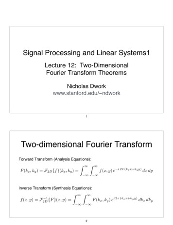
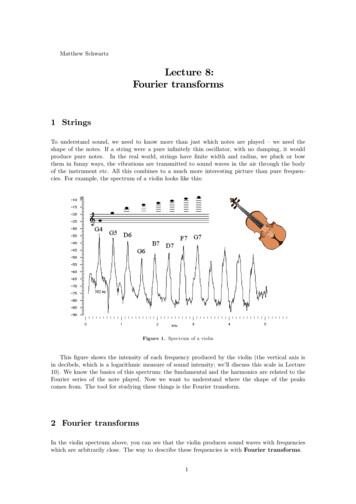
The innermost integral, written here with respect to x1 , is simply the one-dimensionalFourier transform with respect to x1 ; the resulting function is a function of ξ1 , x2 , . . . , xn .Continuing in this manner, we find that the multidimensional transform can be computedwith n independent Fourier transforms, one along each dimension.7Image ProcessingAs we have touched on previously, the Fourier transform has extensive applications to signalprocessing. A number of signal processing techniques, such as filtering, are modeled usingthe convolution of two functions. Since the convolution is very computationally intensive,especially so in higher dimensions, it is common practice to take advantage of the ConvolutionTheorem [2]. If we first compute the transform of each function, multiply the transformedfunctions, and finally compute the inverse transform of their product, the result is exactlythe convolution of the two initial functions.The greatest advantage comes when considering the symmetries of the Fourier transform, allowing us to perform fewer computations for the forward and inverse transforms.Some of these symmetries, along with memory-management techniques, allow a far morecomputationally efficient algorithm for computing the Fourier transform on discrete datasets [3, 4].In the case of image processing, we will consider two-dimensional Fourier transforms. Wecan model a grayscale image as a function f (x), which assigns an intensity value to eachcoordinate x (x1 , x2 ) in the plane. (A full-color image can be treated as a triplet of suchfunctions, one for each of the red, green, and blue channels in the image.) As is often thecase when relating our equations to physical phenomena, this will be a real-valued functionwith a range [0, 1]; a value of 0 represents black pixels and 1 represents a white pixel. Thetransformed function F (ξ) assigns a value to each spatial frequency pair ξ (ξ1 , ξ2 ). Here,interpreting these elements as vectors introduces the notion of a direction for the planarwave described by the corresponding sinusoid, as seen in Figure 1.An illustrative example is beneficial to understanding how the Convolution Theoremapplies to image processing. Let f (x) again be a grayscale image. We consider some functionh(x) that acts as a filter function which produces a processed image g(x) (f h)(x). With8
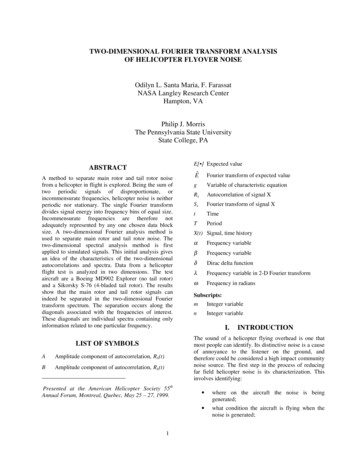
Figure 1: Left to right: Low, intermediate, and high frequency planar waves [5]. The redarrows drawn in image denotes a vector representation of ξ (ξ1 , ξ2 ).the Convolution Theorem, we findg(x) (f h)(x) F 1 [F · H](10)In practice, we care less about h(x) than we do its transform H(ξ); instead we can choosea function H to modify the frequency content of f however we desire [6]. For instance, if wewish to blur the image, we can boost its low frequency content relative to its high frequencies.Similarly, sharpening the image corresponds to increasing its high frequency content relativeto its low frequency content. It is worth noting that the low frequency vectors closest to(ξ1 , ξ2 ) (0, 0) correspond to the overall brightness of the image. This can be seen inFigure 2.We now demonstrate the application of (10). We can define a filter functionH(ξ1 , ξ2 ) ξ1 ξ2 0.3,(11)constructed as a sharpening filter that simultaneously brightens the image. This functionH and the resulting function g are shown in Figure 3. Figures 4-7 showcase various otherfiltering functions and their corresponding output.9
Figure 2: Left: An example input image, representing f (x). Right: The magnitude of thetransformed function F (ξ); the values have been log-scaled to improve visual contrast of thevalues close to zero.Figure 3: Processed image (left) produced by filter H(ξ) ξ1 ξ2 0.3 (right).10
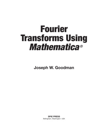
Figure 4: Processed image (left) produced by filter H(ξ) 51 ξ1 (1 ξ2 (right).Figure 5: Processed image (left) produced by filter H(ξ) ξ1 ξ2 (right).11
Figure 6: Processed image (left) produced by filter H(ξ) (1 ξ2 )10 (right).Figure 7: Processed image (left) produced by filter H(ξ) (1 ξ1 )10 (right).12
8Beyond Image ProcessingImage processing problems similar to those posed in eqn. (10) are solved by designing a filterfunction H such that the resulting image g(x) has certain desirable properties. A far moreformidable set of problems are inverse problems [7]. Better stated, given a function g(x),we wish to undo the effects of convolution by some unknown filtering operation to find theoriginal image f (x).There are many physical processes which can be modeled with a convolution that wemay wish undo through solving such an inverse problem. A simple one-dimensional case isthe reconstruction of an audio signal that has been corrupted by noise or other artifacts.In imaging, we may wish to correct a photograph that was taken out-of-focus. Many portions of medical imaging, especially 3-dimensional imaging techniques such as computedtomography (CT) or magnetic resonance imaging (MRI), are dependent on undoing a convolution introduced by the physical imaging process. The resulting function obtained is athree-dimensional reconstruction of the imaging field [8].The solutions to many inverse problems can sometimes be ill-posed since artifacts andnoise introduced by audio recording or imaging can include non-linear terms [7]. Theseinverse problems are then solved as optimization problems, where we wish to find a reconstructed function with the understanding that, in most cases, it will not be identical tothe original function. For any hope of a useful solution, it is essential to have a thoroughunderstanding of the physical processes being modeled.13
References[1] Allan Pinkus and Samy Zafrany. Fourier Series and Integral Transforms. CambridgeUniversity Press, 1997.[2] William H. Press. Numerical Recipes 3rd Edition: The Art of Scientific Computing.Cambridge University Press, sep 2007.[3] James W. Cooley and John W. Tukey. An algorithm for the machine calculation ofcomplex fourier series. Mathematics of Computation, 19(90):297–301, 1965.[4] Matteo Frigo and Steven G. Johnson. The design and implementation of FFTW3. Proceedings of the IEEE, 93(2):216–231, 2005. Special issue on “Program Generation, Optimization, and Platform Adaptation”.[5] B. Osgood. Lecture Notes for EE 261: The Fourier Transform and its Applications.Stanford Engineering Everywhere, 2007.[6] G. L. Zeng. Revisit of the Ramp Filter.62(1):131–136, Feb 2015.IEEE Transactions on Nuclear Science,[7] M. T. McCann, K. H. Jin, and M. Unser. A review of convolutional neural networks forinverse problems in imaging. 2017.[8] A. Myagotin, A. Voropaev, L. Helfen, D. Hänschke, and T. Baumbach. Efficient volumereconstruction for parallel-beam computed laminography by filtered backprojection onmulti-core clusters. IEEE Transactions on Image Processing, 22(12):5348–5361, Dec2013.14
AMATLAB Script% predefined image sizes 512;% load image fileinput imread(’imgs/input.png’);% take 2D FFTfreq fft2(input,s,s);% create absolute value arrayslo ifftshift([0:(s/2-1) (s/2):-1:1]./(s/2));hi ifftshift([(s/2):-1:1 0:(s/2-1)]./(s/2));% create 2D filter functionsfilter horz repmat(lo,s,1);filter vert repmat(lo’,1,s);filter edge hi’*hi;filter shrp hi’*hi 0.3;filter blur lo’*lo;filter blur10 filter blur. 10;% multiply and inverse transformpost vert ifft2(filter vert. 10 .* freq);post horz ifft2(filter horz. 10 .* freq);post shrp ifft2(filter shrp .* freq);post edge ifft2(filter edge .* freq);post blur ifft2(filter blur .* freq);post blur5 ifft2(filter blur. 5 .* freq);15
% postprocess to normalize [0,1]post freq abs(freq) - min(min(abs(freq)));post freq post freq ./ max(max(post freq));post flog log(abs(freq));post flog post flog - min(min(post flog));post flog post flog ./ max(max(post flog));post vert post vert - min(min(post vert));post vert post vert ./ max(max(post vert));post horz post horz - min(min(post horz));post horz post horz ./ max(max(post horz));post shrp post shrp - min(min(post shrp));post shrp post shrp ./ max(max(post shrp));post edge post edge - min(min(post edge));post edge post edge ./ max(max(post edge));post blur post blur - min(min(post blur));post blur post blur ./ max(max(post blur));post blur5 post blur5 - min(min(post blur5));post blur5 post blur5 ./ max(max(post blur5));16
sional Fourier transform; in particular, we consider the 2-dimensional transform and its use in image processing and other problems. We include an example of a typical image processing task an