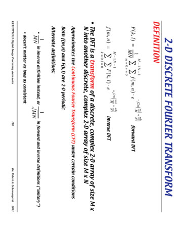
Transcription
2D Fourier Transform
Overview Signals as functions (1D, 2D)– Tools 1D Fourier Transform– Summary of definition and properties in the different cases CTFT, CTFS, DTFS, DTFT DFT 2D Fourier Transforms– Generalities and intuition– Examples– A bit of theory Discrete Fourier Transform (DFT) Discrete Cosine Transform (DCT)
Signals as functions1. Continuous functions of real independent variables–––1D: f f(x)2D: f f(x,y) x,yReal world signals (audio, ECG, images)2. Real valued functions of discrete variables–––1D: f f[k]2D: f f[i,j]Sampled signals3. Discrete functions of discrete variables––––1D: y y[k]2D: y y[i,j]Sampled and quantized signalsFor ease of notations, we will use the same notations for 2 and 3
Images as functions Gray scale images: 2D functions– Domain of the functions: set of (x,y) values for which f(x,y) is defined : 2D lattice[i,j] defining the pixel locations– Set of values taken by the function : gray levels Digital images can be seen as functions defined over a discrete domain {i,j:0 i I, 0 j J}– I,J: number of rows (columns) of the matrix corresponding to the image– f f[i,j]: gray level in position [i,j]
Example 1: δ functioni j 0 1 0δ [i , j ] i , j 0; i j 1 0δ [i , j J ] i 0; j Jotherwise
Example 2: GaussianContinuous functionf ( x, y ) 1eσ 2πx2 y22σ 2Discrete version1f [i , j ] eσ 2πi2 j22σ 2
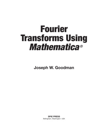
Example 3: Natural image
Example 3: Natural image
Fourier Transform Different formulations for the different classes of signals– Summary table: Fourier transforms with various combinations ofcontinuous/discrete time and frequency variables.– Notations: CTFT: continuous time FTDTFT: Discrete Time FTCTFS: CT Fourier Series (summation synthesis)DTFS: DT Fourier Series (summation synthesis)P: periodical signalsT: sampling periodωs: sampling frequency (ωs 2π/T)For DTFT: T 1 ωs 2π
1D FT: basics
Fourier Transform: Concept A signal can be represented as aweighted sum of sinusoids. Fourier Transform is a change ofbasis, where the basis functionsconsist of sines and cosines(complex exponentials).
Fourier Transform Cosine/sine signals are easy to define and interpret. However, it turns out that the analysis and manipulation of sinusoidalsignals is greatly simplified by dealing with related signals called complexexponential signals. A complex number has real and imaginary parts: z x j y A complex exponential signal:r e jα r ( cos α j sin α )
OverviewTransformTimeFrequency(Continuous Time)Fourier Transform(CTFT)CC(Continuous Time)Fourier Series (CTFS)CAnalysis/SynthesisDualityF (ω ) f (t )e jωt dtSelf-dualt1jω t()f (t ) Fωedω2π ω DPT /21F [k ] f (t )e j 2π kt / T dt T T / 2Dual withDTFTf (t ) F [k ]e j 2π kt / TkDiscrete Time FourierTransform (DTFT)DCPF (ejω tDDPPDual withCTFSnf [ n] Discrete Time FourierSeries (DTFS)) f [n]e j 2πω n / ωsωs / 21ωs F ( e jωt ) e j 2πω n / ωs d ω ωs / 21 N 1F [k ] f [n]e j 2π kn / TN n 0N 1f [n] F [k ]e j 2π kn / Tn 0Self dual
DualitiesSIGNAL DOMAINFOURIER ngSampling PeriodicityDTFS/DFTSampling Periodicity
Discrete time signals Sequences of samples Sampled signals f[k]: sample values f(kTs): sample values Assumes a unitary spacing amongsamples (Ts 1) The sampling interval (or period) is Ts Non normalized frequency ω Transform Normalized frequency Ω Transform––– ––––DTFT for NON periodic sequencesCTFS for periodic sequencesDFT for periodized sequencesAll transforms are 2π periodic DTFTCSTFDFTBUT accounting for the fact that thesequence values have been generatedby sampling a real signal fk f(kTs)All transforms are periodic with periodωsΩ ωTs
CTFT Continuous Time Fourier Transform Continuous time a-periodic signal Both time (space) and frequency are continuous variables– NON normalized frequency ω is used Fourier integral can be regarded as a Fourier series with fundamentalfrequency approaching zero Fourier spectra are continuous– A signal is represented as a sum of sinusoids (or exponentials) of allfrequencies over a continuous frequency intervalFourier integralF (ω ) f (t )e jωt dtanalysis1jω tf (t ) Fedωω() 2π ωsynthesist
CTFT: change of notations Fourier Transform of a 1D continuous signalF (ω ) f ( x)e jω x dx “Euler’s formula”e jω x cos (ω x ) j sin (ω x ) Inverse Fourier Transform1f ( x) 2πChange of notations: F (ω )e jω x d ω ω 2π u ω x 2π u ω y 2π v
Then CTFT becomes Fourier Transform of a 1D continuous signal F (u ) f ( x)e j 2π ux dx “Euler’s formula”e j 2π ux cos ( 2π ux ) j sin ( 2π ux ) Inverse Fourier Transform f ( x) F (u )e j 2π ux du
CTFS Continuous Time Fourier Series Continuous time periodic signals– The signal is periodic with period T0– The transform is “sampled” (it is a series)our notationsT /21 0 jnω0 t()Dn ftedtT oT0 T0 / 2fT0 (t ) Dn e jnω0t2πω0 T0ntable notationsT /21 j 2π kt / TF [k ] ftedt() T T / 2f (t ) F [k ]e j 2π kt / Tkfundamental frequencyT0 TDn F[k]
CTFS Representation of a continuous time signal as a sum of orthogonalcomponents in a complete orthogonal signal space– The exponentials are the basis functions Fourier series are periodic with period equal to the fundamental in the set(2π/T0) Properties– even symmetry only cosinusoidal components– odd symmetry only sinusoidal components
CTFS: example 1
CTFS: example 2
From sequences to discrete time signals Looking at the sequence as to a set of samples obtained by sampling a realsignal with frequency ωs we can still use the formulas for calculating thetransforms as derived for the sequences by– Stratching the time axis (and thus squeezing the frequency axis if Ts 1)normalized frequency(sample series)spectral periodicity in ΩΩ ωTs2π ωs frequency (sampled signal)2πTsspectral periodicity in ω– Enclosing the sampling interval Ts in the value of the sequence samples (DFT)f k Ts f ( kTs )
DTFT Discrete Time Fourier Transform Discrete time a-periodic signal The transform is periodic and continuous with periodour notationsF (Ω) table notations F ( e jω ) f [n]e j 2πω n / ωsf [k ]e jΩkk 1f [k ] 2πnormalizedfrequencyΩ0 2π π F ( Ω )e2nj ΩkdΩf [ n] 1ωsωs / 2 ω Ω F ( Ω ) Fc TΩ ωTs s Ts 2π / ωs Ts 2π / ωssF ( e jωt ) e j 2πω n / ωs d ω/2non normalizedfrequency
Discrete Time Fourier Transform (DTFT) F(Ω) can be obtained from Fc(ω) by replacing ω with Ω/Ts. Thus F(Ω) isidentical to Fc(ω) frequency scaled by a factor 1/Ts– Ts is the sampling interval in time domain Notations Ω F ( Ω ) Fc Ts 2π2πωs Ts ωsTsω Ω Ω ωTsTsperiodicity of the spectrumnormalized frequency (the spectrum is 2π-periodic)F (Ω) F (ωTs ) F ( 2πω / ωs )F (Ω) k f [k ]e j Ωk F (ωTs ) F (ω ) k f [k ]e j 2 kπω / ωs
DTFT: unitary frequency(ω 2π f )Ω 2π uF (Ω) f [k ]e j Ωk F (u ) k 1f [k ] 2π π2 f [k ]e j 2π kuk F (Ω)e jΩk d Ω f [ k ] F (u )e j 2π ku du j 2π ku Fufke()[] k 1 2 f [k ] F (u )e j 2π ku du 1 2112 F (u )e j 2π ku du12NOTE: when Ts 1, Ω ω and the spectrum is2π-periodic. The unitary frequency u 2π/ Ωcorresponds to the signal frequency f 2π/ω.This could give a better intuition of thetransform properties.
Connection f(kTs)0 Ts4Tst0f[k]0 14k02π/TsωF(Ω)2πΩ
Differences DTFT-CTFT The DTFT is periodic with period Ωs 2π (or ωs 2π/Ts) The discrete-time exponential ejΩk has a unique waveform only for values ofΩ in a continuous interval of 2π Numerical computations can be conveniently performed with the DiscreteFourier Transform (DFT)
DTFS Discrete Time Fourier Series Discrete time periodic sequences of period N0– Fundamental frequencyΩ 0 2π / N 0our notations1Dr N0f [k ] table notationsN 0 1 f [k ]e jr Ω0 kk 0N 1N 0 1 Der 01 N 1F [ k ] f [n]e j 2π kn / TN n 0rjr Ω0 kf [k ] F [ k ]e j 2π kn / Tn 0
Discrete Fourier Transform (DFT)Fr N 0 1 k 01fk N0Ω0 f k e jrΩ0 k N 0 1jr Ω0 kFe rk 0N 0 1 k 0 jfk e1 N02πrkN0N 0 1 Fek 0jr2πkN0r2πN0 The DFT transforms N0 samples of a discrete-time signal to the same number ofdiscrete frequency samples The DFT and IDFT are a self-contained, one-to-one transform pair for a length-N0discrete-time signal (that is, the DFT is not merely an approximation to the DTFT asdiscussed next) However, the DFT is very often used as a practical approximation to the DTFT
DFT0kN0zero padding02π/N0F(Ω)2π4πr
Discrete Cosine Transform (DCT) Operate on finite discrete sequences (as DFT) A discrete cosine transform (DCT) expresses a sequence of finitely manydata points in terms of a sum of cosine functions oscillating at differentfrequencies DCT is a Fourier-related transform similar to the DFT but using only realnumbers DCT is equivalent to DFT of roughly twice the length, operating on real datawith even symmetry (since the Fourier transform of a real and even functionis real and even), where in some variants the input and/or output data areshifted by half a sample There are eight standard DCT variants, of which four are common Strong connection with the Karunen-Loeven transform– VERY important for signal compression
DCT DCT implies different boundary conditions than the DFT or other relatedtransforms A DCT, like a cosine transform, implies an even periodic extension of theoriginal function Tricky part– First, one has to specify whether the function is even or odd at both the left andright boundaries of the domain– Second, one has to specify around what point the function is even or odd In particular, consider a sequence abcd of four equally spaced data points, and say thatwe specify an even left boundary. There are two sensible possibilities: either the data iseven about the sample a, in which case the even extension is dcbabcd, or the data iseven about the point halfway between a and the previous point, in which case the evenextension is dcbaabcd (a is repeated).
Symmetries
DCTXk N 0 1 n 02xn N0 π 1 xn cos n k 2 N0 k 0,., N 0 1N 0 1 1 π k 1 X 0 X k cos k 2 k 0 N0 2Warning: the normalization factor in front of these transform definitions is merely aconvention and differs between treatments.–Some authors multiply the transforms by (2/N0)1/2 so that the inverse does not require anyadditional multiplicative factor. Combined with appropriate factors of 2 (see above), this can be used to make the transform matrixorthogonal.
Sinusoids Frequency domain characterization of signalsF (ω ) f (t )e jωt dt Signal domainFrequency domain
Gaussian
rectsinc function
Images vs Signals1D2D Signals Images Frequency Frequency––TemporalSpatial Time (space) frequencycharacterization of signals Reference space for––––FilteringChanging the sampling rateSignal analysis .–Spatial Space/frequency characterization of2D signals Reference space for––––––FilteringUp/Down samplingImage analysisFeature extractionCompression .
2D spatial frequencies 2D spatial frequencies characterize the image spatial changes in thehorizontal (x) and vertical (y) directions– Smooth variations - low frequencies– Sharp variations - high frequenciesyωx 1ωy 0ωx 0ωy 1x
2D Frequency domainωyLarge verticalfrequencies correspondto horizontal linesSmall horizontal andvertical frequenciescorrespond smoothgrayscale changes inboth directionsLarge horizontal andvertical frequenciescorrespond sharpgrayscale changes inboth directionsωxLarge horizontalfrequencies correspondto vertical lines
Vertical gratingωy0ωx
Double gratingωy0ωx
Smooth ringsωyωx
2D box2D sinc
Margherita Hacklog amplitude of the spectrum
Einsteinlog amplitude of the spectrum
What we are going to analyze 2D Fourier Transform of continuous signals (2D-CTFT)1D F (ω ) f (t )e jωt dt , f (t ) F (ω )e jωt dt 2D Fourier Transform of discrete space signals (2D-DTFT)1DF (Ω) f [k ]e j Ωkk 1, f [k ] 2π πF (Ω)e jΩk dt22D Discrete Fourier Transform (2D-DFT)1DFr N0 1 f [k ]ek 0 jrΩ0 k1 N0 1 jrΩ0k2π, f N0 [k ] ,FeΩ r0N0 r 0N0
2D Continuous Fourier Transform Continuous case (x and y are real) – 2D-CTFT (notation 1)fˆ (ω x , ω y ) f ( x, y ) e j (ω x x ω y y )dxdy f ( x, y ) 14π 2 j (ω x ω y )fˆ (ω x , ω y ) e x y d ω x d ω y f ( x, y ) g * ( x, y ) dxdy f g 1fˆ (ω x , ω y )gˆ * (ω x , ω y ) d ω x d ω y Parseval formula4π 2 221f ( x, y ) dxdy 2 fˆ (ω x , ω y ) d ω x d ω y4πPlancherel equality
2D Continuous Fourier Transform Continuous case (x and y are real) – 2D-CTFTω x 2π uω y 2π vfˆ ( u , v ) f ( x, y ) e j 2π ( ux vy ) dxdy f ( x, y ) 14π 214π 2 2fˆ ( u , v ) e j 2π ( ux vy ) ( 2π ) dudv ˆf ( u , v ) e j 2π ( ux vy ) ( 2π )2 dudv
2D Continuous Fourier Transform 2D Continuous Fourier Transform (notation 2)fˆ ( u , v ) f ( x, y ) e j 2π ( ux vy ) dxdy f ( x, y ) fˆ ( u , v ) e j 2π ( ux vy ) dudv f ( x, y ) dxdy 2 2fˆ (u , v) dudvPlancherel’s equality
2D Discrete Fourier TransformThe independent variable (t,x,y) is discreteFr N 0 1 f [ k ]e jrΩ0 kF [u , v] 2πΩ0 N0 f [i, k ]e jΩ0 ( ui vk )i 0 k 0k 01f N0 [k ] N0N 0 1 N 0 1N 0 1 r 0Fr e jrΩ0 k1f N0 [i, k ] 2N02πΩ0 N0N 0 1 N 0 1 u 0 v 0F [u , v]e jΩ0 ( ui vk )
Delta Sampling property of the 2D-delta function (Dirac’s delta) δ ( x x , y y ) f ( x, y)dxdy f ( x , y )0000 Transform of the delta functionF {δ ( x, y )} j 2π ( ux vy )δ(x,y)edxdy 1 F {δ ( x x0 , y y0 )} j 2π ( ux vy ) j 2π ( ux vy )δ(x x,y y)edxdy e00 00shiftingproperty
Constant functions Inverse transform of the impulse function F 1 {δ (u , v)} j 2π ( ux vy )j 2π (0 x v 0)δ(u,v)edudv e 1 Fourier Transform of the constant ( 1 for all x and y)k ( x, y ) 1F {k } x, y j 2π ( ux vy )edxdy δ (u , v)
Trigonometric functions Cosine function oscillating along the x axis– Constant along the y axiss( x, y ) cos(2π fx)F {cos(2π fx)} j 2π ( ux vy )πfxedxdy cos(2) e j 2π ( fx ) e j 2π ( fx ) j 2π (ux vy ) dxdy e2 1 e j 2π (u f ) x e j 2π (u f ) x e j 2π vy dxdy 2 11 e j 2π vy dy e j 2π (u f ) x e j 2π (u f ) x dx 1 e j 2π (u f ) x e j 2π ( u f ) x dx 2 2 1[δ (u f ) δ (u f )]2
Vertical gratingωy-2πf02πfωx
Ex. 1
Ex. 2
Ex. 3Magnitudes
Examples
Properties Linearityaf ( x, y ) bg ( x, y ) aF (u , v) bG (u , v) j 2π ( ux0 vy0 ) Shiftingf ( x x0 , y x0 ) e Modulatione j 2π ( u0 x v0 y ) f ( x, y ) F (u u0 , v v0 ) Convolutionf ( x, y ) * g ( x, y ) F (u , v)G (u , v) Multiplicationf ( x, y ) g ( x, y ) F (u , v) * G (u , v) Separabilityf ( x, y ) f ( x) f ( y ) F (u, v) F (u ) F (v)F (u, v)
Separability1. Separability of the 2D Fourier transform– 2D Fourier Transforms can be implemented as a sequence of 1D FourierTransform operations performed independently along the two axis F (u , v) f ( x, y )e j 2π (ux vy ) dxdy f ( x, y ) e j 2π ux j 2π vye dxdy F (u, y)e e j 2π vy j 2π vy dy f ( x, y )e j 2π ux dx dy F ( u, v ) 2D DFT1D DFT alongthe rows1D DFT alongthe cols
Separability Separable functions can be written as f ( x, y ) f ( x ) g ( y )2. The FT of a separable function is the product of the FTs of the two functions F (u , v) f ( x, y )e j 2π ( ux vy ) dxdy h( x ) g ( y ) e H (u ) G (v ) j 2π ux j 2π vye dxdy g ( y)e j 2π vy dy h( x)e j 2π ux dx f ( x, y ) h ( x ) g ( y ) F ( u , v ) H ( u ) G ( v )
2D Fourier Transform of a Discrete function Fourier Transform of a 2D a-periodic signal defined over a 2D discrete grid– The grid can be thought of as a 2D brush used for sampling the continuoussignal with a given spatial resolution (Tx,Ty)1DF (Ω ) f [k ]e jΩk , f [ k ] k 2DF (Ω x , Ω y ) f [k ] 14π 2 k1 k2 π πΩx,Ωy: normalized frequency2πf [k1 , k2 ]eF (Ω x , Ω y )e2 2 F (Ω)e jΩk dt j ( k1Ω x k2 Ω y ) 12πj ( k1Ω x k2 Ω y )d ΩxΩ y
Unitary frequency notations Ω x 2π u Ω y 2π vF (u, v) k1 k2 1/ 2 1/ 2f [k1 , k2 ] f [k1 , k2 ]e j 2π ( k1u k2v )F (u , v)e j 2π ( k1u k2v ) dudv 1/ 2 1/ 2 The integration interval for the inverse transform has width 1 instead of 2π–It is quite common to choose 11 u, v 22
Properties Periodicity: 2D Fourier Transform of a discrete a-periodic signal is periodic– The period is 1 for the unitary frequency notations and 2π for normalizedfrequency notations.– Proof (referring to the firsts case)F (u k , v l ) f [m, n]e j 2π ( ( u k ) m ( v l ) n )1m n Arbitraryintegers f [m, n]e j 2π ( um vn ) j 2π km j 2π lnem n m n F (u , v)f [m, n]e j 2π (um vn )e1
Properties Linearity shifting modulation convolution multiplication separability energy conservation properties also exist for the 2D Fourier Transform ofdiscrete signals. NOTE: in what follows, (k1,k2) is replaced by (m,n)
2D DTFT Properties Linearityaf [m, n] bg[m, n] aF (u , v) bG (u , v) Shiftingf [m m0 , n n0 ] e j 2π (um0 vn0 ) F (u , v) Modulationej 2π ( u0 m v0 n )f [m, n] F (u u0 , v v0 ) Convolutionf [m, n]* g[m, n] F (u , v)G (u , v) Multiplicationf [m, n]g[m, n] F (u , v) * G (u , v) Separable functionsf [m, n] f [m] f [n] F (u , v) F (u ) F (v) Energy conservation m n 1/ 2 1/ 2f [m, n] 2 1/ 2 1/ 22F (u, v) dudv
Impulse Train Define a comb function (impulse train) as followscombM , N [m, n] δ [m kM , n lN ]k l where M and N are integers1comb2 [n]n
Appendix
2D-DTFT: delta Define Kronecker delta function 1, for m 0 and n 0 δ [m, n] 0, otherwise DT Fourier Transform of the Kronecker delta functionF (u , v) j 2π ( um vn ) j 2π ( u 0 v 0 ) 1δ[m,n]ee m n
2D DT Fourier Transform: constant Fourier Transform of 1f [k , l ] 1, k , lF [u , v] j 2π ( uk vl ) 1e k l δ (u k , v l )k l periodic with period 1along u and vTo prove: Take the inverse Fourier Transform of the Dirac delta function and use the fact thatthe Fourier Transform has to be periodic with period 1.
Fourier Transform of a 1D continuous signal Ffxedx() ()ω jxω Inverse Fourier Transform 1 ( ) 2 fx F e dω jxω ω π “Euler’s formula” exjx jxω cos sin(ω) (ω) Change of notations: