Transcription
Fourier transforms and convolution(without the agonizing pain)CS/CME/BioE/Biophys/BMI 279Oct. 14, 2021Ron Dror1
Outline Why do we care? Convolution– Moving averages– Mathematical definition Fourier transforms– Writing functions as sums of sinusoids– The Fast Fourier Transform (FFT)– Multi-dimensional Fourier transforms Performing convolution using Fourier transforms2
Why do we care?3
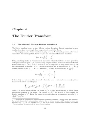
Why study Fourier transforms andconvolution? In the remainder of the course, we’ll study severalmethods that depend on analysis of images orreconstruction of structure from images:– Light microscopy (particularly fluorescence microscopy)– Cryoelectron microscopy– X-ray crystallography The computational aspects of each of thesemethods involve Fourier transforms and convolution These concepts also underlie algorithms used for– Ligand docking and virtual screening– Molecular dynamics simulations
Convolution5A more descriptive name than convolution would be “weighted moving average”
Pollution (measured value)A function, as stored in a computerTime (minutes)
Time (minutes)Pollution (true value)
ConvolutionMoving averages8
Pollution (measured value)Original data (measurements)Time (minutes)
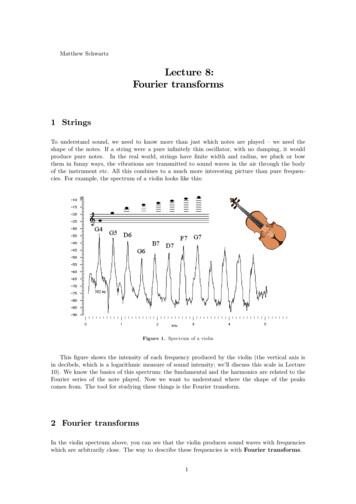
Moving averageCalled a “moving” average,because you average thevalues surrounding yourdata point of interestPollution (moving average)Weighting function(equal weights)Time (minute)Areas of fast change (ie when time is between 4-8 minutes) can have problems!
Weighted moving averagePollution (moving average)Weighting function(unequal weights)Time (minutes)Using a weighting function is less noisy and allows you to better estimate areas of fast change
A convolution is basically aweighted moving average We’re given an array of numerical values– We can think of this array as specifying values of a function atregularly spaced intervals To compute a moving average, we replace each value inthe array with the average of several values that precedeand follow it (i.e., the values within a window) We might choose instead to calculate a weighted movingaverage, where we again replace each value in the arraywith the average of several surrounding values, but weweight those values differently We can express this as a convolution of the originalfunction (i.e., array) with another function (array) thatspecifies the weights on each value in the window12
Examplef function of measurementg weighting functionf convolved with g (written f g) Same as g convolved with f13
ConvolutionMathematical definition14
Convolution: mathematical definition If f and g are functions defined at evenly spacedpoints, their convolution is given by: ( f g )[ n ] f [ m ]g [ n m ]m 15
ConvolutionMultidimensional convolution16
Images as functions of two variables Many of the applications we’llconsider involve images A grayscale image can bethought of as a function oftwo variables– The position of each pixelcorresponds to some value of xand y– The brightness of that pixel isproportional to f(x,y)yx17
Two-dimensional convolution In two-dimensional convolution, we replace eachvalue in a two-dimensional array with a weightedaverage of the values surrounding it in twodimensions– We can represent two-dimensional arrays as functionsof two variables, or as matrices, or as images18
Two-dimensional convolution: examplefgf g (f convolved with g)19
Multidimensional convolution The concept generalizes to higher dimensions For example, in three-dimensional convolution,we replace each value in a three-dimensionalarray with a weighted average of the valuessurrounding it in three dimensions20
Fourier transforms21
Fourier transformsWriting functions as sums of sinusoids22
Sinusoid waveWriting functions as sums of sinusoids Given a function defined on an interval of length L,we can write it as a sum of sinusoids whose periodsare L, L/2, L/3, L/4, (plus a constant term)Original function Starting and ending values (x -50, and x 50) are sameSum of sinusoids below Decreasing periodIncreasing frequency 23
Writing functions as sums of sinusoids Given a function defined on an interval of length L,we can write it as a sum of sinusoids whose periodsare L, L/2, L/3, L/4, (plus a constant term)Original functionsum of 49 sinusoids (plus constant term)sum of 50 sinusoids (plus constant term)24
You can do this for any function!Writing functions as sums of sinusoids Each of these sinusoidal terms has a magnitude(scale factor) and a phase (shift).Original functionSum of sinusoids belowMagnitude: Howhigh the peaks arePhase: x position offirst maximum Magnitude: -0.3Phase: 0 (arbitrary) Magnitude: 1.9Phase: -.94 Magnitude: 0.27Phase: -1.4Magnitude: 0.39Phase: -2.8
Expressing a function as a set ofsinusoidal term coefficients We can thus express the original function as aseries of magnitude and phase coefficients– If the original function is defined at N equally spacedpoints, we’ll need a total of N coefficients– If the original function is defined at an infinite set ofinputs, we’ll need an infinite series of magnitude andphase coefficients—but we can approximate thefunction with just the first fewConstant term(frequency 0)Magnitude: -0.3Phase: 0 (arbitrary)Sinusoid 1(period L, frequency 1/L)Magnitude: 1.9Phase: -.94Sinusoid 2(period L/2, frequency 2/L)Magnitude: 0.27Phase: -1.4Sinusoid 3(period L/3, frequency 3/L)Magnitude: 0.39Phase: -2.8
Using complex numbers to representmagnitude plus phase We can express the magnitude and phase ofeach sinusoidal component using a complexnumber Complex number a single numberwith a real term and a imaginary termImaginary partMagnitude lengthof blue arrowPhase angle of blue arrowRealpart
Using complex numbers to representmagnitude plus phase We can express the magnitude and phase ofeach sinusoidal component using a complexnumber Thus we can express our original function as aseries of complex numbers representing thesinusoidal components– This turns out to be more convenient (mathematicallyand computationally) than storing magnitudes andphases
The Fourier transform The Fourier transform maps a function to a set ofcomplex numbers representing sinusoidalcoefficients– We also say it maps the function from “real space” to“Fourier space” (or “frequency space”)– Note that in a computer, we can represent a function asan array of numbers giving the values of that function atequally spaced points. The inverse Fourier transform maps in the otherdirection– It turns out that the Fourier transform and inverseFourier transform are almost identical. A program thatcomputes one can easily be used to compute the other.
Why do we want to express our functionusing sinusoids? Sinusoids crop up all over the place in nature– For example, sound is usually described in terms ofdifferent frequencies Sinusoids have the unique property that if yousum two sinusoids of the same frequency (of anyphase or magnitude), you always get anothersinusoid of the same frequency– This leads to some very convenient computationalproperties that we’ll come to later30
Fourier transformsThe Fast Fourier Transform (FFT)31
The Fast Fourier Transform (FFT)Fourier transforms become computationally intense with large number of data points The number of arithmetic operations required tocompute the Fourier transform of N numbers(i.e., of a function defined at N points) in astraightforward manner is proportional to N2 Surprisingly, it is possible to reduce this N2 toNlogN using a clever algorithm– This algorithm is the Fast Fourier Transform (FFT)– It is arguably the most important algorithm of the pastcentury– (For this class, you’re not required to know just howthis algorithm works, although it’s really interesting!) 32
Fourier transformsMultidimensional Fourier Transforms33
Images as functions of two variables Many of the applications we’llconsider involve images A grayscale image can bethought of as a function oftwo variables– The position of each pixelcorresponds to some value of xand y– The brightness of that pixel isproportional to f(x,y)yx34
Two-dimensional Fourier transform We can express functions of two variables as sums of sinusoids Each sinusoid has a frequency in the x-direction and a frequencyin the y-direction We need to specify a magnitude and a phase for each sinusoid Thus the 2D Fourier transform maps the original function to acomplex-valued function of two frequenciesOn the left, the sinusoid isplotted as a surface, while f ( x, y ) sin ( 2π 0.02x 2π 0.01y )the right, the sinusoidalfunction is shown as animage35
Three-dimensional Fourier transform The 3D Fourier transform maps functions of threevariables (i.e., a function defined on a volume) toa complex-valued function of three frequencies 2D and 3D Fourier transforms can also becomputed efficiently using the FFT algorithm36
Performing convolution using Fouriertransforms37
Relationship between convolution andFourier transforms It turns out that convolving two functions isequivalent to multiplying them in the frequencydomain– One multiplies the complex numbers representingcoefficients at each frequency In other words, we can perform a convolution bytaking the Fourier transform of both functions,multiplying the results, and then performing aninverse Fourier transform38
Why does this relationship matter? First, it allows us to perform convolution faster– If two functions are each defined at N points, thenumber of operations required to convolve them in thestraightforward manner is proportional to N2– If we use Fourier transforms and take advantage of theFFT algorithm, the number of operations isproportional to NlogN Second, it allows us to characterize convolutionoperations in terms of changes to differentfrequencies– For example, convolution with a Gaussian willpreserve low-frequency components while reducinghigh-frequency components39
Three-dimensional Fourier transform The 3D Fourier transform maps functions of three variables (i.e., a function defined on a volume) to a complex-valued function of three frequencies 2D and 3D Fourier transforms ca