WIXLIB

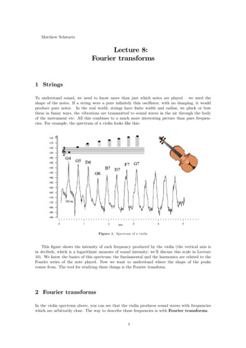
Matthew SchwartzLecture 8:Fourier transforms1 StringsTo understand sound, we need to know more than just which notes are played – we need theshape of the notes. If a string were a pure infinitely thin oscillator, with no damping, it wouldproduce pure notes. In the real world, strings have finite width and radius, we pluck or bowthem in funny ways, the vibrations are transmitted to sound waves in the air through the bodyof the instrument etc. All this combines to a much more interesting picture than pure frequencies. For example, the spectrum of a violin looks like this:Figure 1. Spectrum of a violinThis figure shows the intensity of each frequency produced by the violin (the vertical axis isin decibels, which is a logarithmic measure of sound intensity; we’ll discuss this scale in Lecture10). We know the basics of this spectrum: the fundamental and the harmonics are related to theFourier series of the note played. Now we want to understand where the shape of the peakscomes from. The tool for studying these things is the Fourier transform.2 Fourier transformsIn the violin spectrum above, you can see that the violin produces sound waves with frequencieswhich are arbitrarily close. The way to describe these frequencies is with Fourier transforms.1

2Section 2Recall the Fourier exponential series Xf (x) cne2π n xLi(1)n where1cn LZL2dxf (x)eL i2πn xL(2) 2To check this, we plug Eq. (1) into Eq. (2) giving1cn LZL2Ldx 2" Xcmei2π m xLm #e2πn xL i 1 XLcmm ZL2Ldxei2π m xLe i2πn xL(3) 2Then using the mathematical identityZL2L 22πdxei (m n) x L Lδm n(4)cmLδn m cn(5)2πnL(6)we getcn 1 XLm as desired. That is, we have checked Eq. (2).To derive the Fourier transform, we writekn where n is still an integer going from to . For arbitrary L, kn can get arbitrarily big inthe positive or negative direction. However, at fixed L, the lowest non-zero kn cannot be arbi2πtrarily small: kn L . Then, we defineLc1f (kn) n 2π2πZL2Ldxf (x)e ikn x(7) 2The factor of 2π in this equation is just a convention. Now we can take L so that kn canget arbitrarily close to zero. This gives1f (k) 2πZ dxf (x)e ikx(8) where now k can be any real number. This is the Fourier transform. It is a continuum generalization of the cn’s of the Fourier series.The inverse of this comes from writing Eq. (1) as a integral. From Eq. (6), we find d kn This leads to2π n.Lf (x) Xn cneikx n Xn cneikxLdkn 2πZ dk f (k)eikx where we have used Eq. (7) and taken L in the last step.(9)

3ExampleSo we have1f (k) 2πZ dxf (x)e ikx f (x) Z dk f (k)ei kx(10) We say that f (k) is the Fourier transform of f (x). The factor of 2π is just a convention. Wecould also have defined f (x) with the 2π in it. The sign on the phase is also a convention (that1 R is, we could have defined f (k) 2π d xf (x)ei kx instead). Keep in mind that different conventions are used in different places and by different people. There is no universal convention forthe 2π factors. All conventions lead to the same physics.The Fourier transform of a function of x gives a function of k, where k is the wavenumber.The Fourier transform of a function of t gives a function of ω where ω is the angular frequency:1f (ω) 2πZ dtf (t)e iωt(11) 3 ExampleAs an example, let us compute the Fourier transform of the position of an underdamped oscillator:f (t) e γtcos(ω0t)θ(t)(12)where the unit-step function is defined byθ(t) 1,0,t 0t60(13)This function insures that our oscillator starts at time t 0. If didn’t include, the amplitudewould blow up as t .We first write11f (t) e γtcos(ω0t)θ(t) e γteiω0tθ(t) e γte iω0tθ(t)22(14)So we can Fourier transform the simpler exponential function. Starting with the first term, wefindZ1 dte γte i (ω ω0) tθ(t)f ω0(ω) 4π Z1 dte( γ i ω iω0)t4π 0 11e( γ iω iω0)t 4π γ i(ω ω0)011 4π γ i(ω ω0)In the last step we have used that the t endpoint vanishes due to the e γt factor and thatat the t 0 endpoint the exponential is 1. The second term in Eq. (14) is the first term withω0 ω0. Thus the full Fourier transform is 1111ω iγ (15)f (ω) 2πi (ω iγ)2 ω024π γ i(ω ω0) γ i(ω ω0)

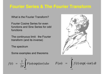
4Section 4As mentioned before, the spectrum plotted for an audio signal is usually f (ω) 2. Let’s see whatthis looks like. We’ll take ω0 10 and γ 2. The function and the modulus squared f (ω) 2 ofits Fourier transform are then:Figure 2. An underdamped oscillator and its power spectrum (modulus of its Fourier transformsquared) for γ 2 and ω0 10.We now can also understand what the shapes of the peaks are in the violin spectrum in Fig.1. The widths of the peaks give how much each harmonic damps with time. The width at halfmaximum gives the damping factor γ.4 Fourier transform is complexFor a real function f (t), the Fourier transform will usually not be real. Indeed, the imaginarypart of the Fourier transform of a real function is Z Z f (k) f (k) 1 1 i kxikx Im f (k) dxf (x)e dxf (x)e 2i2i 2π 12πZ(16) dxf (x)sin(kx) f s(k)(17)This is a Fourier sine transform. Thus the imaginary part vanishes only if the function has nosine components which happens if and only if the function is even. For an odd function, theFourier transform is purely imaginary. For a general real function, the Fourier transform willhave both real and imaginary parts. We can writef (k) f c(k) if s(k)(18)where f s(k) is the Fourier sine transform and f c(k) the Fourier cosine transform. One hardlyever uses Fourier sine and cosine transforms. We practically always talk about the complexFourier transform.Rather than separating f (k) into real and imaginary parts, which amounts to Cartesiancoordinates, it is often helpful to write it as a magnitude and phase, as in polar coordinates. Sowe writef (k) A(k)ei φ(k)with A(k) f (k) the magnitude and φ(k) the phase.(19)

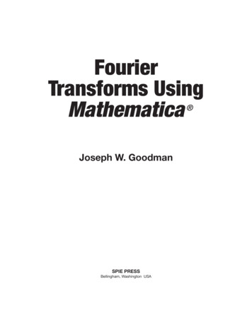
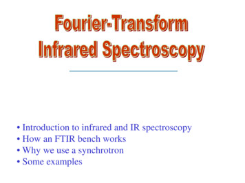
5Fourier transform is complexThe energy in a frequency mode only depends on the amplitude: I A(ω)2. When one plotsthe spectrum as in audacity, what is being shown is A(ω)2. This corresponds to the intensity orpower in a particular mode, as we will see in Lecture 10. Power is useful in doing a frequencyanalysis of sound since it tells us how loud that frequency is. But looking at the amplitude isnot the only thing one can do with a Fourier transform. Often one is also interested in thephase.For a visual example, we can take the Fourier transform of an image. Suppose we have agrayscale image that is 640 480 pixels. Each pixel is a number from 0 to 255, going from black(0) to white (255). Thus the image is a function f (x, y) with 0 6 x 640, 0 6 y 480 whichtakes values from 0 to 255. We can then Fourier transform this function to a function f (kx , k y):ZZ 1 dxdy f (x, y)e ikx xe k yy(20)f (kx , k y) 2π The 2D Fourier transform is really no more complicated than the 1D transform – we just do twointegrals instead of one. So what we do we get? Here’s an exampleImage fpanda (x, y)Magnitude, Apanda (kx , k y)Phase φpanda (kx , k y)Figure 3. Fourier transform of a panda. The magnitude is concentrated near kx k y 0, corresponding tolarge-wavelength variations, while the phase looks random.We can do the same thing for a picture of a cat:Image fcat (x, y)Magnitude, Acat (kx , k y)Phase φcat (kx , k y)Figure 4. Fourier transform of a cat. The magnitude is concentrated near kx k y 0, but maybe not asmuch as the panda, since that cat has smaller wavelength features. Phase still looks random.Now let’s Fourier transform back. Of course for the cat and panda we get back the orignalimage. But what happens if we combine the magnitude for the panda with the phase for thecat, and vice versa?

6Section 5Acat (kx , k y) and φpanda (kx , k y)Apanda (kx , k y) and φcat (kx , k y)Figure 5. We take the inverse Fourier transform of function Aca t (kx , k y )eiφpanda(kx ,k y) on the left, andAp a n d a (kx , k y)eiφcat(kx,k y) on the right.It looks like the phase is more important than the magnitude for reconstructing the originalimage. The importance of phase is critical for many engineering applications, such as signalanalysis. It is also relevant for image compression technologies.5 FilteringOne thing we can do with the Fourier transform of an image is remove some components. If weremove low frequencies, less than some ωf say, we call it a high-pass filter. A lot of background noise is at low frequencies, so a high-pass filter can clean up a signal. If we throw outthe high frequencies, it is called a low-pass filter. A low pass filter can be used to smooth data(such as a digital photo) since it throws out high frequency noise. A filter that cuts out bothhigh and low frequencies is called a band-pass filter.Here are some examplesphoto of EinsteinPhoto after high-pass filterFigure 6. What a high-pass filter does to Albert Einstein.

7Filteringphoto of EinsteinPhoto after low-pass filterFigure 7. What a low-pass filter does to Marylyn Monroe.Now let’s combine the twohigh-pass Einstein low pass Marylynlow-pass Einstein high-pass MarylynFigure 8. Combining filtered imagesTake a look at these last two images from up close and from far away. What do you see?Why?

8Section 66 Dirac δ functionAnother extremely important example is the Fourier transform of a constant:Z1 dte iωtδ(ω) 2π Its Fourier inverse is thenZ 1 dωδ(ω)eiωt(21)(22) This object δ(ω) is called the Dirac δ function. It is enormously useful in a great variety ofphysics problems, especially in quantum mechanics, but also in waves.To figure out what δ(ω) looks likes, we use the fact that the Fourier transform of the inverseFourier transform gives a function back. That is, for any smooth function f (x)f (x) Z dkeikxf (k) Z dy Z12πZ12πZ dkeikx Z dyf (y)e ik y(23) dke ik(y x) f (y)(24) dyδ(y x)f (y)(25)where we used Eq. (21) in the last step. Setting x 0, we see that the δ-function satisfiesZ dxδ(x)f (x) f (0)(26) for any smooth function f (x). δ(x) also has the property that δ(x) 0 for x / 0 (see Section 6.1below), so thatZ x0dxδ(x)f (x) f (0)(27) x0for any x0.Eq. (26) and (27) uniquely define the δ-function. Indeed, the δ-function is no ordinary function. It is instead a member of a class of mathematical objects called distributions. Whilefunctions take numbers and give numbers (like f (x) x2), distributions only give numbers afterbeing integrated.You should think of δ(x) as zero everywhere except at x 0 where it is infinite. However,R xthe infinity is integrable: x0 δ(x) 1 for any x0 0.0From the physics point of view, we showed that if we have an amplitude which is constant intime f (t) 1 then the only frequency mode supported has 0 frequency. This makes sense – aconstant has an infinite wavelength and never repeats. Conversely, if f (ω) 1 it says that allfrequencies are excited. This corresponds to white noise. The Fourier transform of f (ω) 1gives a function f (t) δ(t) which corresponds to an infinitely sharp pulse. For a pulse has nocharacteristic time associated with it, no frequency can be picked out. That’s why white noisehas all frequencies equally.6.1 Some mathematics of δ(ω) (optional)For ω / 0 the quickest way to evaluate δ(ω) integral is by contour integration. If you’ve neverseen any complex analysis, just ignore this section. If you have, consider the integral in the com-