Transcription
FourierTransforms UsingMathematica Joseph W. GoodmanSPIE PRESSBellingham, Washington USA
Fourier Transforms Using Mathematica 1Fourier Transforms Using MathematicaJoseph W. GoodmanStanford UniversityPrefaceThis book is a product of shelter-in-place. During the spring of 2020, when COVID-19 was rampant, staying inside and isolated was therecommended way to avoid infection. Under such circumstances, the mind seeks activities that will keep one occupied and stimulated. Theactivity of choice for me was writing a book on Fourier transforms using Mathematica.Fourier transforms is a subject quite familiar to me. I had taught a graduate-level course on this subject for many years at Stanford, sometimeswith more than 100 students coming from departments across the university. During this time I accumulated substantial lecture notes, uponwhich much of this book is based. However, this book does contain some material that was not included in the classes I taught.Mathematica is a program I used extensively in illustrating other books, but I was by no means an expert on its capabilities. I took thecombination of Fourier transforms and Mathematica as a challenge, and indeed I learned a great deal about this program in the course ofwriting this material. Still I do not consider myself a Mathematica expert, but rather a user who loves to find capabilities of this program that Ihave not yet discovered. Hopefully the reader of this book will emerge as a reasonably knowledgeable user of the program.I learned Fourier transforms first as a graduate student in a course on the subject taught at Stanford by Ron Bracewell, a well-known radioastronomer and an innovator in many fields. In addition to his well-known books on Fourier transforms, he wrote a compendium on theEucalyptus trees on the Stanford campus. He was a true renaissance man. His course shaped my career, and in gratitude, I am dedicating thisbook to his memory.Table of Contents1. Introduction1.1 Why Mathematica?1.2 What the Reader Should Know at the Start1.3 Why Study the Fourier Transform?2. Some Useful 1D and 2D Functions2.1 User-Defined Names for Useful Functions2.2 Dirac Delta Functions2.3 The Comb Function3. Definition of the Continuous Fourier Transform3.1 The 1D Fourier Transform and Inverse Fourier Transform3.2 The 2D Fourier Transform and Inverse Fourier Transform3.3 Fourier Transform Operators in Mathematica3.4 Transforms in-the-Limit3.5 A Table of Some Frequently Encountered Fourier Transforms4 Convolutions and Correlations4.1 Convolution Integrals4.2 The Central Limit Theorem4.3 Correlation Integrals5. Some Useful Properties of Fourier Transforms5.1 Symmetry Properties of Fourier Transforms5.2 Area and Moment Properties of 1D Fourier Transforms5.3 Area and Moment Properties of 2D Fourier Transforms5.4 Fourier Transform Theorems5.5 The Projection-Slice Theorem5.6 Widths in the x and u Domains
25. Some Useful Properties of Fourier Transforms5.1 Symmetry Properties of Fourier Transforms5.2 Area and Moment Properties of 1D Fourier Transforms5.3 Area and Moment Properties of 2D Fourier Transforms5.4 Fourier Transform Theorems5.5 The Projection-Slice Theorem5.6 Widths in the x and u Domains6. Fourier Transforms in Polar Coordinates6.1 Using the 2D Fourier Transform for Circularly Symmetric Functions6.2 The Zero-Order Hankel Transform6.3 The Projection-Transform Method6.4 Polar-Coordinate Functions with a Simple Harmonic Phase7. Linear Systems and Fourier Transforms7.1 The Superposition Integral for Linear Systems7.2 Linear Invariant Systems and the Convolution Integral7.3 Transfer Functions of Linear Invariant Systems7.4 Eigenfunctions of Linear Invariant Systems8. Sampling and Interpolation8.1 The Sampling Theorem in One Dimension8.2 The Sampling Theorem in Two Dimensions9. From Fourier Transforms to Fourier Series9.1 Periodic Functions and Their Fourier Transforms9.2 Example of a Complex Fourier Series9.3 Mathematica Commands for Fourier Series9.4 Other Types of Fourier Series9.5 Circular Harmonic Expansions10. The Discrete Fourier Transform10.1 Sampling in Both Domains10.2 Vectors and Matrices in Mathematica10.3 The Discrete Fourier Transform (DFT)10.4 The DFT and Mathematica10.5 DFT Properties and Theorems10.6 Discrete Convolutions and Correlations10.7 The Fast Fourier Transform (FFT)11. The Fresnel Transform11.1 Definition of the 1D Fresnel Transform11.2 Approximations to the Bandwidth of the Interval-Limited Quadratic-Phase Exponential11.3 Equivalent Bandwidth of the Interval-Limited Quadratic-Phase Exponential11.4 The 2D Fresnel Transform11.5 The Fresnel Transform of Circularly Symmetric Functions11.6 Examples of Fresnel Transforms11.7 The Fresnel-Diffraction Transfer Function11.8 The Discrete Fresnel-Diffraction Integral12. Fractional Fourier Transforms12.1 Definition of the Fractional Fourier Transform12.2 Mathematica Calculation of the Fractional Fourier Transform12.3 Relationship between the Fractional Fourier Transform and the Fresnel-Diffraction Integral13. Other Transforms Related to the Fourier Transform13.1 The Abel Transform13.2 The Radon Transform13.3 The Hilbert Transform13.4 The Analytic Signal13.5 The Laplace Transform13.6 The Mellin Transform
13. Other Transforms Related to the Fourier Transform13.1 The Abel Transform13.2 The Radon Transform13.3 The Hilbert Transform13.4 The Analytic Signal13.5 The Laplace Transform13.6 The Mellin TransformFourier Transforms Using Mathematica 314. Fourier Transforms and Digital Image Processing with Mathematica14.1 Inputting an Image Into Mathematica14.2 Some Elementary Properties of Images14.3 Some Image Point Manipulations14.4 Blurring and Sharpening Images in Mathematica14.5 Fourier Domain Processing of Images15. Fourier Transforms and Mathematica in Coherent Optical Systems15.1 Background on Fourier Transforms in Coherent Optical Systems15.2 Optical Fourier-Domain Filtering15.3 Phase Contrast Imaging15.4 Digital Phase-Stepping Holography15.5 Simulation of Speckle in Coherent ImagingAppendix A: Proofs of Fourier Transform TheoremsAppendix B: Proof of the Uncertainty PrincipleReferences1. IntroductionThe Fourier transform is a ubiquitous tool used in most areas of engineering and physical sciences. The purpose of this book is two-fold: 1) tointroduce the reader to the properties of Fourier transforms and their uses, and 2) to introduce the reader to the program Mathematica and todemonstrate its use in Fourier analysis. Unlike many other introductory treatments of the Fourier transform, this treatment will focus from thestart on both one-dimensional (1D) and two-dimensional (2D) transforms, the latter of which play an important role in optics and digital imageprocessing, as well as in many other applications. It is hoped that by the time the reader has completed this book, he or she will have a basicfamiliarity with both Fourier analysis and Mathematica.1.1 Why MathematicaMany other texts on Fourier transforms exist, especially notable among them being those by Bracewell [1], Papoulis [2], and, for a more recentbook, Osgood [3]. This book differs from others in that it is devoted to exploring these topics with the help of the program Mathematica. Thebook has been written as a Mathematica notebook, allowing the reader to interact with the document using the free program Wolfram Player.Considering the various computational languages available, why have we chosen Mathematica here? The reasons are several. First, Mathematica seamlessly blends symbolic and numerical mathematics, with incredibly broad knowledge about various functions and capabilities. Second,Mathematica allows the creation of documents such as this, which include both mathematical computations and formatted text. Finally, if thereader has the full Mathematica program (rather than just Wolfram Player), he or she can change the various commands that are executed inthis ebook and explore other functions, other parameters, etc.Mathematica is the creation of Stephen Wolfram and the company Wolfram Research. It was first released in 1988, and has appeared in manyversions. This book was written using version 12. There are many books that cover the capabilities of Mathematica; see for example, Mathematica Navigator by H. Ruskeepaa, and The Student's Introduction to Mathematica and the Wolfram Language by B.F. and E.A. Torrence, twoamong many. In addition, the Wolfram documentation available under the Mathematica help menu contains all you need to know aboutindividual commands and their syntax.Mathematica is an extremely powerful language with a huge number of commands. In general, commands have names that to some extentreveal their function. It is possible to write very dense and compact code in this language, but in this book we have chosen to sacrificecompactness for understandability. Thus the calculations presented here can often be written in more compact forms, but those forms will beharder to understand than the forms we have used here.An attempt has been made to limit the number of Mathematica commands used in this book to a subset of the available commands, simply asan aid to the reader. The syntax and actions of these commands are covered in detail in the references and in the Mathematica Help menu, asare also the syntax and actions of many other commands that have not been used here.
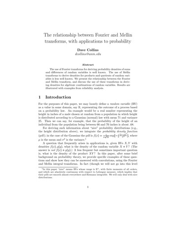
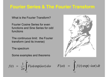
5Fourier Transforms Using Mathematica There are several reasons for studying Fourier transforms. First, it is likely to be your most important mathematical tool in problem solving,regardless of your specialty in physics or engineering. Second, it provides a valuable bridge between your chosen area of expertise and otherareas of engineering and physics. To illustrate the ubiquitous nature of Fourier transforms: they are used by circuit designers for studying thefrequency response of circuits; they are used by radio astronomers to form images from interferometric data gathered with antenna arrays; theyare used by spectroscopists to obtain high-resolution spectra in the infrared from interferograms, a method known as Fourier spectroscopy; theyare used by crystallographers to find crystal structure using Fourier transforms of X-ray diffraction patterns; and they are used by cameradesigners to specify camera performance in terms of spatial frequency response. Even psychologists have used Fourier transforms in the studyof memory and perception. Almost regardless of your field, you will be able to use your knowledge of Fourier transforms to your advantage.Back to Contents?2. Some Useful 1D and 2D Functions2.1 User-Defined Names for Useful FunctionsOur interest here will be in both 1D and 2D functions and their transforms. As a start it is useful to define a group of 1D functions. 2Dfunctions can be built using these functions. By a 1D function, we mean one that is defined on a line. By a 2D function, we mean one that isdefined on a plane. The following table provides a set of 1D functions that have user-defined names (all beginning with lower-case letters) andthe corresponding Mathematica code that defines those functions. Again, these definitions are included in an initialization cell near thebeginning of this document.rect[x ] : UnitBox[x];sinc[x ] : Sinc Pi * x ;step[x ] : UnitStep[x];sgn[x ] : Sign[x];gaus[x ] : Exp - Pi * x 2 ;jinc[x ] : 2 * BesselJ 1, Pi * x Pi * x ;tri[x ] : UnitTriangle[x];rtri[x ] : rect[x - 1 / 2] * UnitTriangle[x];δ[x ] : DiracDelta[x];comb[x ] : DiracComb[x];A table showing plots of most of these functions follows. The functions δ(x) and comb(x) will be discussed in Section 2.5. Note that thecommand to plot such functions isPlot[g[x], {x, lower, upper}, PlotRange All],where lower and upper are the lower and upper limits, respectively, for which the function should be ri[x]jinc[x]
10and in two dimensions - An important important property is that comb(ax) g(x, y) comb(x, y) ⅆ x ⅆ y g(n, m).m - n - 11a2combx.aBack to Contents?3. Definition of the Continuous Fourier Transform3.1 The 1D Fourier Transform and Inverse TransformWe begin with a discussion of 1D Fourier transforms. We start with a function g(x) defined on the x axis, and calculate its 1D transform 4(u)defined on the u axis. There are several possible definitions of the Fourier transform, differing through scaling constants applied to thetransform and/or to its argument. Mathematica defines the 1D Fourier transform 4(u) of the function g(x) through the equationb4(u) (2 π)1-a g(x) exp(ⅈ b u x) ⅆ x ,- where a and b are the scaling constants to be chosen. The symbol ⅈ represents the imaginary constant -1 , while a and b are called theFourier parameters. The symbol x may represent time, in which case the symbol u represents temporal frequency, measured in hertz (Hz).The definition of the transform to be used here and throughout is one that chooses the constants (a, b) (0, –2π), yielding4(u) - g( x) exp(-ⅈ 2 π u x) ⅆ x . This equation now has to be expressed in Mathematica language. The expression that performs this operation on an input function g(x) is:[u ] : FourierTransform g[x], x, u, FourierParameters 0, - 2 * Pi Notice the underbar following u in the definition of the function 4, as is required in any definition of a function in Mathematica. Notice alsothe delayed equality symbol : , which means that the expression will not be evaluated until it is needed in later code.Paralleling the definition of the Fourier transform is that of the inverse Fourier transform. Mathematica’s definition of this quantity isg(x) b(2 π)1 a - 4(u) exp (–ⅈ b u x) ⅆu. To return from 4 to g given our definition of the transform requires that we again choose the Fourier parameters for the inverse transform as {a,b} {0, –2π}. We then obtain g(x) 4(u) exp(ⅈ 2 π u x) ⅆ u.- This equation can be thought of as expressing g(x) as a superposition of an infinite number of weighted complex exponentials of the form 4(u)exp(ⅈ 2 π u x), where 4(u) is the weighting function for the complex exponential with frequency u. The Mathematica command to perform theinverse Fourier transform is given byg[x ] : InverseFourierTransform :[u], u, x, FourierParameters - 0, - 2 * Pi For all but the most unusual functions, the inverse Fourier transform of the Fourier transform of a function g(x) returns the function g(x), exceptat points of discontinuity of g, where the average of the values of g from the right and from the left of the discontinuity is obtained. Discussionof the conditions for successful inversion of the Fourier transform by the inverse Fourier transform will follow later.3.2 The 2D Fourier Transform and Inverse TransformIn this text, we shall often consider 2D functions that are defined on an (x, y) spatial plane. The Fourier transforms of such functions arelikewise 2D functions defined on a frequency plane. Again there are several different definitions of the 2D transform that differ from oneanother through scaling of the transform or the frequency variables, or both. Mathematica defines the 2D Fourier transform through theequation
14Back to Contents?4. Convolutions and CorrelationsIn many fields of physics and engineering, the convolution integral and the correlation integral play important roles in analysis. In this chapterwe explore these integrals in one and two dimensions, and discuss their implementations in Mathematica.4.1 Convolution IntegralsThe convolution g(x) between two functions h(x) and f(x) is defined by the integral g( x ) f (ξ) h(x - ξ) ⅆ ξ f (x) * h(x).- Here the symbol ξ is simply a dummy variable of integration, and the symbol * stands for convolution between the two stated functions. (Donot confuse this symbol with the multiplication symbol used in Mathematica code.) Note that one of the functions, in this case h(ξ), has beenreversed left to right and shifted to be centered at ξ x. The same resulting g(x) is obtained if f(ξ), rather than h(ξ), is reversed and shifted.Consider the case of functions f(x) gaus(x) and h(ξ) rtri(x). Both functions are shown below:Visualizing the area under the convolution integral can be accomplished with the Mathematica command Manipulate. The form of thiscommand isManipulate expression , a, amin, amax .Note that to use this command, you must enable “Dynamic Updating” in the Evaluation menu. If the resulting plot shows only an outline of thecoordinate system, highlight the cell marker for the command on the right and execute the command by pressing shift-return, assuming you areusing the full Mathematica program.This expression allows one, for example, to plot a function with a variable parameter, and to visualize the changes in the function as theparameter is varied. In the present case, the command needed is
Fourier Transforms Using Mathematica In[! ]: 15Manipulate Plot gaus[x], rtri[- x a], gaus[x] * rtri[- x a] , {x, - 1, 2},PlotRange All, ExclusionsStyle Automatic, AxesLabel {x, None},Filling Axis, FillingStyle Automatic , {a, - 0.9, 1.6}, SaveDefinitions True aOut[! ] In this plot, axis labels are explicitly called for, and the curves are colored down to the x axis. By moving the button above the plot, the overlapof the two functions being convolved changes, and the reader can see the integrand of the convolution integral plotted.Mathematica has a command for convolving two functions f and h:g[x ] Convolve f[ξ], h[ξ], ξ, x .As an example, consider the convolution of the right half-triangle with a scaled version of itself:In[! ]: g[x ] Convolve rtri[2 * ξ], rtri[ξ], ξ, x 124Out[! ] 161(7 - 6 x)124(- 3 2 x)23 x 11 x x 6 - 9 x 2 x2 0 x 03212TrueThe result is quite complex, but it can be visualized with a plot:In[! ]: Plot[g[x], {x, - 1.5, 2.0}, AxesLabel {x, "g(x )"}]g(x)0.150.10Out[! ] 0.05-1.5-1.0-0.50.51.01.52.0x
20In[! ]: Plot3D c[x, y], {x, - 1, 0.5}, {y, - 1, 0.5},PlotRange All, PlotPoints 40, AxesLabel {x, y, "c[x,y]"} Out[! ] You should be aware that in some cases Mathematica is unable to find the convolution or the correlation. For example,In[! ]: c[x ] Convolve jinc[ξ], jinc[- ξ], ξ, x 4 Convolve BesselJ[1,π ξ]Out[! ] ξ,BesselJ[1,π ξ]ξ, ξ, x π2We note that it is often still possible to find the correlation function by reasoning in the frequency domain using the autocorrelation theoremdescribed in the Section 5.4.Back to Contents?5. SomeUsefulTransformsPropertiesofFourierFourier transforms have a number of interesting properties that are of great help in analyzing problems. In this chapter we discuss some ofthese properties in detail. Our attention is limited to properties for which Mathematica is helpful or relevant.5.1 Symmetry Properties of Fourier TransformsSymmetry properties in the x domain result in other symmetry properties in the u domain; we explore these properties in this section.Every function g(x) can be written as the sum of an even part e(x) and an odd part o(x), whereg(x) e(x) o(x),e(x) g(x) g(-x)2,o( x ) g(x) - g(-x)2and this decomposition is unique. However, the decomposition does depend on the origin chosen for g(x). For example, cos(x) is even, butcos(x – π/2) sin(x) is odd.Consider now the symmetry properties of the Fourier transform 4(u) that result when we impose symmetry properties on g(x). The Fouriertransform of g(x) can be written as 4(u) (e( x) o( x)) (cos(2 π u x) - ⅈ sin(2 π u x)) ⅆ x - - - - - e(x) cos(2 π u x) ⅆ x - ⅈ e(x) sin(2 π u x) ⅆ x o(x) cos(2 π u x) ⅆ x - ⅈ o(x) sin(2 π u x) ⅆ x,where we have expanded the complex exponential into a sum of a real cosine term and an imaginary sine term.The infinite integral of any function that is odd in x will vanish. Note that e(x) sin(2πux) and o(x) cos(2πux) are both odd functions in x, andtherefore their integrals vanish, leaving two integrals with integrands that are even functions of x,
Fourier Transforms Using Mathematica 4(u) - 21 e(x) cos(2 πux) ⅆ x - ⅈ o(x) sin(2 πux) ⅆ x.- From this set of two integrals we can determine the properties of the even and odd parts of 4(u) by focusing on their u dependencies. The tablebelow shows the resulting symmetry properties of 4(u):g ( x)4 ( u)even and realeven and realeven and imaginary even and imaginaryodd and realodd and imaginaryodd and imaginaryodd and realWe conclude from this table that when g(x) is real, we have 4(–u) 4* (u) and we say that 4(u) has Hermitian symmetry, while when g(x) isimaginary, 4(–u) –4* (u) and we say that 4(u) has anti-Hermitian symmetry. Note also that when g(x) is even, the symmetry properties of4(u) are the same as the symmetry properties of g(x), while when g(x) is odd, they are not the same.We illustrate these properties with two examples: g(x) tri(x)*sgn(x), an odd and real function, and ⅈtri(x), an even and imaginary function:In[! ]: ft1 tri[x] * sgn[x] ⅈ - 2 π u Sin[2 π u] Out[! ] In[! ]: Out[! ] 2 π2 u2ft1 I * tri[x] ⅈ Sinc[π u]2In the first example, we see that the transform is odd and imaginary, as predicted, while in the second example the transform is even andimaginary, also as predicted.5.2 Area and Moment Properties of 1D Fourier TransformsThere is an intimate relationship between moments of functions in the x domain and the behavior of their Fourier transforms at the origin in thefrequency domain. The simplest of these relations is an “area” property (the zeroth-order moment). According to this property, - g(x) ⅆ x lim g(x) e-ⅈ2πux ⅆ x 4(0).u 0 - To verify this theorem using Mathematica, we first integrate the Gaussian function to find its area, and then calculate the value of its Fouriertransform at the origin. The two commands follow.In[! ]: Out[! ] In[! ]: Out[! ] Integrate gaus[x], x, - Infinity, Infinity 1Limit ft1[gaus[x]], u 0 1The equality of these two quantities holds for any function that is absolutely integrable. It also holds for most transforms in-the-limit.There exist related correspondences between moments of functions in the x domain and derivatives of their Fourier transforms at the origin inthe frequency domain. Assuming that xk g(x) ⅆ x , - starting with the frequency domain expression and moving to the x domain,ⅈ2πⅈ Thus,2πk Lim g(x)u 0- ⅆkⅆukkLimu 0e-ⅈ2πux ⅆ x ⅆkkⅆuⅈ2π g(x) e-ⅈ2πux ⅆ x- kLim u 0 - -ⅈ2πux(-ⅈ2π x)k g( x) e ⅆx - xk g(x) ⅆ x.
Fourier Transforms Using Mathematica 27The following examples of the first, second, and third derivatives of gaus[x] may be helpful:First derivative:In[! ]: Clear[:1, :2, :3]:1[u ] ft1[D[gaus[x], {x, 1}]]2Out[! ] 2 ⅈ ⅇ-π u π uSecond derivative:In[! ]: :2[u ] ft1[D[gaus[x], {x, 2}]]2Out[! ] - 4 ⅇ-π u π2 u2Third derivative:In[! ]: :3[u ] ft1[D[gaus[x], {x, 3}]]2Out[! ] - 8 ⅈ ⅇ-π u π3 u3You can see that in each case the spectrum is indeed as predicted above. Note that for every odd derivative, the result for a real 4(u) isimaginary, while for every even derivative, the result for a real 4(u) is real-valued.In[! ]: Plot {Im[:1[u]], :2[u], Im[:3[u]]}, {u, - 2, 2}, PlotRange All,PlotLegends "Expressions", FillingStyle Automatic, AxesLabel {u, None} Im('1(u))'2(u)Out[! ] Im('3(u))The command PlotLegends- Automatic plots a legend next to the figure. Note that Mathematica can even find an expression for the nthderivative of the Gaussian function, although it takes some time to compute:In[! ]: Out[! ] ft1[D[gaus[x], {x, n}]]2-1 n ⅇⅈnπ2-π u21--nAbs[u]-1 nπ - u Abs[u] u Abs[u] Cos[n π] u Abs[u] Erfi π Abs[u] Sin[n π] In this result, the Erfi function is the so-called “imaginary error function,” described in the Mathematica Help menu under Wolframdocumentation.The derivative theorem also works in reverse, i.e., for derivatives in the frequency domain. The relationship in this reverse direction isⅆkⅆuk4(u) (-ⅈ2π x)k g( x).5.5 The Projection-Slice TheoremThe projection-slice theorem is sufficiently important to warrant its own section. This theorem states that given a projection (to be definedbelow) through a 2D function g(x, y) at angle θ to the x axis, the 1D Fourier transform of that projection is a central slice through the 2Dspectrum of g(x, y) at angle θ to the u axis in the frequency domain. Projections are at the heart of computerized tomography systems used inmedical X-ray and MRI machines.
48In[! ]: Clear[c, d, e]c[n ] (1 / 3) * ft1 tri[x] * rect[x / 3] /. u n / 3;Quiet[d Table[c[n], {n, - 10, 10}]];d[[11]] Limit[c[n], n 0];e Table Exp I * 2 * Pi * (n / 3) * x , {n, - 10, 10} ;NPlot d.e, {x, - 4, 4}, Filling Axis, AxesLabel x, "g (x )" g,(x)1.00.80.6Out[! ] 0.40.2-4-224xThis has been our first exposure to lists in Mathematica. We will encounter them in much more detail when we consider the discrete Fouriertransform in the next chapter.9.3 Mathematica Commands for Fourier SeriesIn the section above, we have shown the relations between Fourier transforms and complex Fourier series, including methods for constructingsuch series given one period of a periodic function. Mathematica actually has a set of commands that make these calculations much easier. Inwhat follows, we keep the same definition of the function p(x) defining one period, i.e., p(x) tri(x) rect(x/3).The most useful Mathematica command with respect to complex Fourier series is the FourierSeries[p[x],x,n,FourierParameters- {a,b}] command. Mathematica defines this command to find Fourier coefficients ck according tobck 2 π a 12π b - π g(x) ⅇ-ⅈ b k xⅆ x,k -n, ., n. b To have this representation of the ck conform to those derived above, the Fourier parameters (a, b) must be chosen as {1,2*Pi/L}, where Lis the period of the periodic function. We illustrate with the same periodic function used above, for which the period is 3. We choose n 4, aswe did in the first case above.
52In[! ]: FullSimplify f.e 2Out[! ] 35π2 ρ HypergeometricPFQ , 2, , - π2 ρ2 Sin[ϕ]322We can see this result by plotting it. But first we convert it to a function of rectangular coordinates using the commandSqrt[u 2 v 2],ϕ ArcTan[u,v]}. The plot is then:In[! ]: /.{ρ Plot3D f.e /. {ρ Sqrt[u 2 v 2], ϕ ArcTan[u, v]}, {u, - 5, 5},N{v, - 5, 5}, AxesLabel u, v, ":" , PlotRange All, PlotPoints 30 Out[! ] Thus, the cos(θ) variation of the phase and the circ(r) dependence on radius in the (r, θ) plane have created a Fourier transform with a positivemound and a negative mound, due to the sin(ϕ) dependence in the transform plane.Note that, while we have illustrated with a simple function that is separable in polar coordinates, the method also works when the Fouriercoefficients of the phase depend on r, although the computation times can be long.We turn now to the discrete Fourier transform.Back to Contents?10. The Discrete Fourier TransformWhen we are dealing with discrete data, Fourier analysis plays an important role, for both 1D and 2D data. However, the Fourier transformmust be modified to accommodate discrete data rather than continuous data. These modifications are the subject of this chapter.10.1 Sampling in Both DomainsSuppose we wish to estimate the Fourier transform of a physical process f(x) that we imagine has existed from x – and will continue to existin the future for all x. We can measure f(x) only over a limited duration of x, and therefore must base our estimate of the spectrum on a finitesegment,g(x) f ( x) 0 x L0otherwise.Our measurement instruments can only measure samples of g(x), so we must base our spectral estimate on a collection of such samples. Whilea spectrum of a finite duration signal can not be bandlimited, it can be approximately bandlimited to a total bandwidth B, so we can sample withspacing Δx 1/B with minimum aliasing in the spectral domain. As we have seen, the result of this sampling is to replicate the spectrum tocreate a periodic Fourier transform, with a period given by the reciprocal of the sampling interval, i.e., a period of width B or greater if wesample in the x domain with spacing 1/B or smaller.It is not generally possible to calculate a continuous spectrum of g(x), for it would involve computation of an infinite number of spectralsamples spaced infinitesimally apart, so we must also sample the spectrum. Since the data sample is limited to duration L, we can sample thespectrum with spacing Δu 1/L (or finer) without incurring aliasing in the x domain. If we sample in the x domain with the minimum allowable spacing, the number of samples of g(x) will be N L /(1/B) LB.Thus, when dealing with real data, we must work with finite sets of samples in both the x domain and the u domain. The discrete Fouriertransform (DFT) is the tool that allows such spectral estimation to be performed. In this chapter we explore the DFT and its properties.
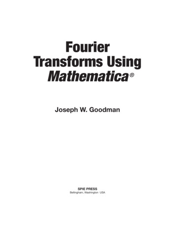
62In[! ]: LogPlot {2 * n 3, 2 * n 2 * Log[2, n]}, {n, 1, 1000},PlotRange {10 0, 10 10}, AxesLabel N, "Operations" ,PlotLegends {"Brute Force", "FFT"}, PlotLabel "Operation Counts vs. N " Operation Counts vs. NOperations108Brute ForceOut[! ] 10FFT510002004006008001000NFor a 1000 1000 image array, the reduction in operations when performing the FFT rather than the brute force DFT is about a factor of 100.This reduction often makes the difference between an uncomfortably long computation and a much more reasonable computation time.Back to Contents?11. The Fresnel TransformA close relative of the Fourier transform is the Fresnel transform, a mathematical operation widely used in signal processing, optics, acoustics,and electromagnetics. In this chapter we explore the Fresnel transform for both continuous functions and discrete data. The 1D Fresneltransform is important in radar signal theory. The 2D Fresnel transform is important in the theory of diffraction of waves of various types.11.1 Definition of the 1D Fresnel TransformThe definitions of the 1D Fresnel transform differ in signal processing and in optics. For signal processing, the 1D Fresnel transform f(
13.6 The Mellin Transform 2. 13. Other Transforms Related to the Fourier Transform 13.1 The Abel Transform 13.2 The Radon Transform 13.3 The Hilbert Transform 13.4 The Analytic Signal 13.5 The Laplace Transform . A table