Transcription
Chapter 4The Fourier Transform4.1The classical discrete Fourier transformThe Fourier transform occurs in many di erent versions throughout classical computing, in areasranging from signal-processing to data compression to complexity theory.For our purposes, the Fourier transform is going to be an N N unitary matrix, all of whoseentries have the same magnitude. For N 2, it’s just our familiar Hadamard transform: 111F2 H p.12 1Doing something similar in 3 dimensions is impossible with real numbers: we can’t give threeorthogonal vectors in { 1, 1}3 . However, using complex numbers allows us to define the Fourierk 1transform for any N . Let !N e2 i/N be an N -th root of unity (“root of unity” means that !Nfor some integer k, in this case k N ). The rows of the matrix will be indexed by j 2 {0, . . . , N 1}jkand the columns by k 2 {0, . . . , N 1}. Define the (j, k)-entry of the matrix FN by p1N !N:01.C1 BjkBFN p @ · · · ! N··· CAN.Note that FN is a unitary matrix, since each column has norm 1, and any two columns (say thoseindexed by k and k 0 ) are orthogonal: NN 1X1 11 X j(k0 k)1 if k k 0jk 1jk0p (!N ) p !N !N 0 otherwiseNNNj 0j 0Since FN is unitary and symmetric, the inverse FN 1 FN only di ers from FN by having minussigns in the exponent of the entries. For a vector v 2 RN , the vector vb FN v is called theFourier transform of v.1 Doing the matrix-vector multiplication, its entries are given by vbj PN 1 jkp1k 0 !N vk .N1The literature on Fourier analysis usually talks about the Fourier transform of a function rather than of a vector,but on finite domains that’s just a notational variant of what we do here: a vector v 2 RN can also be viewed as afunction v : {0, . . . , N 1} ! R defined by v(i) vi . Also, in the classical literature people sometimes use the term“Fourier transform” for what we call the inverse Fourier transform.21
4.2The Fast Fourier TransformThe naive way of computing the Fourier transform vb FN v of v 2 RN just does the matrixvector multiplication to compute all the entries of vb. This would take O(N ) steps (additions andmultiplications) per entry, and O(N 2 ) steps to compute the whole vector vb. However, there is amore efficient way of computing vb. This algorithm is called the Fast Fourier Transform (FFT,due to Cooley and Tukey in 1965), and takes only O(N log N ) steps. This di erence between thequadratic N 2 steps and the near-linear N log N is tremendously important in practice when N islarge, and is the main reason that Fourier transforms are so widely used.We will assume N 2n , which is usually fine because we can add zeroes to our vector to makeits dimension a power of 2 (but similar FFTs can be given also directly for most N that aren’t apower of 2). The key to the FFT is to rewrite the entries of vb as follows:vbj N 11 X jkp!N v kN k 0 1pN 1p2Xjkj!Nv k !Neven k1Xj(k 1)!Nvkodd kXpN/2 even kjk/2!N/2 vk j!N!X1pN/2 odd kj(k 1)/2!N/2vk!Note that we’ve rewritten the entries of the N -dimensional Fourier transform vb in terms of twoN/2-dimensional Fourier transforms, one of the even-numbered entries of v, and one of the oddnumbered entries of v.This suggest a recursive procedure for computing vb: first separately compute the Fourier transform v[even of the N/2-dimensional vector of even-numbered entries of v and the Fourier transformvdodd of the N/2-dimensional vector of odd-numbered entries of v, and then compute the N entries1jvbj p ([vevenj !Nvdoddj ).2Strictly speaking this is not well-defined, because v[even and vdodd are just N/2-dimensional vectors.However, if we define v[[even j N/2 vevenj (and similarly for vdodd ) then it all works out.The time T (N ) it takes to implement FN this way can be written recursively as T (N ) 2T (N/2) O(N ), because we need to compute two N/2-dimensional Fourier transforms and doO(N ) additional operations to compute vb. This recursion works out to time T (N ) O(N log N ),as promised. Similarly, we have an equally efficient algorithm for the inverse Fourier transformFN 1 FN , whose entries are p1N !Njk .4.3Application: multiplying two polynomialsSuppose we are given two real-valued polynomials p and q, each of degree at most d:p(x) dXaj xj and q(x) j 0dXk 022bk x k
We would like to compute the product of these two polynomials, which is01!dd2d X2dXXXjAk@(p · q)(x) aj xbk x (aj b j )x ,j 0k 0 0 j 0 {zc }where implicitly we set aj bj 0 for j d and b j 0 if j . Clearly, each coefficient c byitself takes O(d) steps (additions and multiplications) to compute, which suggests an algorithm forcomputing the coefficients of p · q that takes O(d2 ) steps. However, using the fast Fourier transformwe can do this in O(d log d) steps, as follows.NNThe convolutionPNof 1two vectors a, b 2 R is a vector a b 2 R whose -th entry is defined1by (a b) pN j 0 aj b jmodN . Let us set N 2d 1 (the number of nonzero coefficientsof p · q) and make the above (d 1)-dimensional vectors of coefficients a and b N -dimensional byadding d zeroes. Thenp the coefficients of the polynomial p · q are proportional to the entries of theconvolution: c N (a b) . It is easy to show that the Fourier coefficients of the convolution ofa and b are the products of the Fourier coefficients of a and b: for every 2 {0, . . . , N 1} we havead b ba ·bb . This immediately suggests an algorithm for computing the vector of coefficients c : dapply the FFT to a and b to get ba and bb, multiply those twop vectors entrywise to get a b, applythe inverse FFT to get a b, and finally multiply a b with N to get the vector c of the coefficientsof p · q. Since the FFTs and their inverse take O(N log N ) steps, and pointwise multiplication oftwo N -dimensional vectors takes O(N ) steps, this algorithm takes O(N log N ) O(d log d) steps.Note that if two numbers ad · · · a1 a0 and bd · · · b1 b0 are given in decimal notation, then we caninterpretPtheir digits as coefficientsP of single-variate degree-d polynomials p and q, respectively:p(x) dj 0 aj xj and q(x) dk 0 bk xk . The two numbers will now be p(10) and q(10). Theirproduct is the evaluation of the product-polynomial p · q at the point x 10. This suggests thatwe can use the above procedure (for fast multiplication of polynomials) to multiply two numbers inO(d log d) steps, which would be a lot faster than the standard O(d2 ) algorithm for multiplicationthat one learns in primary school. However, in this case we have to be careful since the steps of theabove algorithm are themselves multiplications between numbers, which we cannot count at unitcost anymore if our goal is to implement a multiplication between numbers! Still, it turns out thatimplementing this idea carefully allows one to multiply two d-digit numbers in O(d log d log log d)elementary operations. This is known as the Schönhage-Strassen algorithm, which is one of theingredients in Shor’s algorithm (see the next chapter). We’ll skip the details.4.4The quantum Fourier transformSince FN is an N N unitary matrix, we can interpret it as a quantum operation, mapping an N dimensional vector of amplitudes to another N -dimensional vector of amplitudes. This is called thequantum Fourier transform (QFT). In case N 2n (which is the only case we will care about), thiswill be an n-qubit unitary. Notice carefully that this quantum operation does something di erentfrom the classical Fourier transform: in the classical case we are given a vector v, written on a pieceof paper so to say, and we compute the vector vb FN v, and also write the result on a piece ofpaper. In the quantum case, we are working on quantum states; these are vectors of amplitudes, butwe don’t have those written down anywhere—they only exist as the amplitudes in a superposition.23
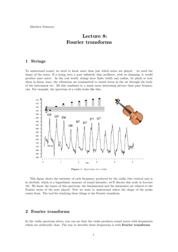
We will see below that the QFT can be implemented by a quantum circuit using O(n2 ) elementarygates. This is exponentially faster than even the FFT (which takes O(N log N ) O(2n n) steps),but it achieves something di erent: computing the QFT won’t give us the entries of the Fouriertransform written down on a piece of paper, but only as the amplitudes of the resulting state.4.5An efficient quantum circuitHere we will describe the efficient circuit for the n-qubit QFT. The elementary gates we will allowourselves are Hadamards and controlled-Rs gates, where 10Rs .s0 e2 i/2 101 0sNote that R1 Z , R2 . For large s, e2 i/2 is close to 1 and hence010 ithe Rs -gate is close to the identity-gate I. We could implement Rs -gates using Hadamards andcontrolled-R1/2/3 gates, but for simplicity we will just treat each Rs as an elementary gate.Since the QFT is linear, it suffices if our circuit implements it correctly on basis states ki, i.e.,it should mapN 11 X jk ki 7! FN ki p!N ji.N j 0The key to doing this efficiently is to rewrite FN ki, which turns out to be a product state (so FNdoes not introduce entanglement when applied to a basis state ki). Let ki k1 P. . . kn i, k1 beingnthe most significant bit. Note that for integer j j1 . . . jn , we can write j/2 n 1 j 2 . Forexample, binary 0.101 is 1·2 1 0·2 2 1·2 3 5/8. We have the following sequence of equalities:FN ki N 11 X 2 ijk/2npe jiN j 0N 11 X 2 i(Pn 1 j 2peN j 0 )k j1 . . . jn iN 1 n1 X Y 2 ij k/2 pe j1 . . . jn iN j 0 1n O1 p 0i e2 ik/2 1i .2 1 Note that e2 ik/2 e2 i0.kn 1 .kn : the n most significant bits of k don’t matter for this value.As an example, for n 3 we have the 3-qubit product state111F8 k1 k2 k3 i p ( 0i e2 i0.k3 1i) p ( 0i e2 i0.k2 k3 1i) p ( 0i e2 i0.k1 k2 k3 1i).222This example suggests what the circuit should be. To prepare the first qubit of the desired stateF8 k1 k2 k3 i, just apply a Hadamard to k3 i, giving state p12 ( 0i ( 1)k3 1i) and observe that24
( 1)k3 e2 i0.k3 . To prepare the second qubit of the desired state, apply a Hadamard to k2 i, givingp1 ( 0i e2 i0.k2 1i), and then conditioned on k3 (before we apply the Hadamard to k3 i) apply R2 .3This multiplies 1i with a phase e2 i0.0k3 , producing the correct qubit p12 ( 0i e2 i0.k2 k3 1i). Finally,to prepare the third qubit of the desired state, we apply a Hadamard to k1 i, apply R2 conditionedon k2 and R3 conditioned on k3 . This produces the correct qubit p12 ( 0i e2 i0.k1 k2 k3 1i). We havenow produced all three qubits of the desired state F8 k1 k2 k3 i, but in the wrong order : the firstqubit should be the third and vice versa. So the final step is just to swap qubits 1 and 3. Figure 4.1illustrates the circuit in the case n 3. Here the black circles indicate the control-qubits for eachof the controlled-Rs operations, and the operation at the end of the circuit swaps qubits 1 and 3.The general case works analogously: starting with 1, we apply a Hadamard to k i and then“rotate in” the additional phases required, conditioned on the values of the later bits k 1 . . . kn .Some swap gates at the end then put the qubits in the right order.2Figure 4.1: The circuit for the 3-qubit QFTSince the circuit involves n qubits, and at most n gates are applied to each qubit, the overallcircuit uses at most n2 gates. In fact, many of those gates are phase gates Rs with slog n, whichare very close to the identity and hence don’t do much anyway. We can actually omit those from thecircuit, keeping only O(log n) gates per qubit and O(n log n) gates overall. Intuitively, the overallerror caused by these omissions will be small (Exercise 4 asks you to make this precise). Finally,note that by inverting the circuit (i.e., reversing the order of the gates and taking the adjoint U of each gate U ) we obtain an equally efficient circuit for the inverse Fourier transform FN 1 FN .4.6Application: phase estimationSuppose we can apply a unitary U and we are given an eigenvector i of U (U i i), andwe would like to approximate the corresponding eigenvalue . Since U is unitary, must havemagnitude 1, so we can write it as e2 i for some real number 2 [0, 1); the only thing thatmatters is this phase . Suppose for simplicity that we know that 0. 1 . . . n can be writtenwith n bits of precision. Then here’s the algorithm for phase estimation:1. Start with 0n i i2. For N 2n , apply FN to the first n qubits to get(in fact, H n I would have the same e ect)2p12nPN1k 0 ki iWe can implement a SWAP-gate using CNOTs (Exercise 2.4); CNOTs can in turn be constructed from Hadamardand controlled-R1 ( controlled-Z) gates, which are in the set of elementary gates we allow here.25
3. Apply the map ki i 7! kiU k i e2 i k ki i. In other words, apply U to the secondregister for a number of times given by the first register.4. Apply the inverse Fourier transform FN 1 to the first n qubits and measure the result.P 1 2 i kNote that after step 3, the first n qubits are in state p1N N ki FN 2n i, hence thek 0 einverse Fourier transform is going to give us 2n i 1 . . . n i with probability 1.In case cannot be written exactly with n bits of precision, one can show that this procedurestill (with high probability) spits out a good n-bit approximation to . We’ll omit the calculation.Exercises1. For ! e2 i/3010 1011 1101and F3 p13 @ 1 ! ! 2 A, calculate F3 @ 1 A and F3 @ ! 2 A1 !2 !0!2. Prove that the Fourier coefficients of the convolution of vectors a and b are the product ofthe Fourier coefficients of a and b. In other words, prove that for every a, b 2 RN and every 2 {0, . . . , N 1} we have ad b ba · bb . Here the Fourier transform ba is defined as the PN 11vector FN a, and the -entry of the convolution-vector a b is (a b) pN j 0 aj b jmodN .PP3. The Euclideanpdistancebetween two states i i i ii and i i i ii is defined asP2k i ik i . Assume the states are unit vectors with (for simplicity) reali iamplitudes. Suppose the distance is small: k i ik . Showthen the probabilitiesP that22resulting from a measurement on the two states are also close: ii 2 .iHint: use i22i ii · i i and the Cauchy-Schwarz inequality.4. The operator norm of a matrix A is defined as kAk max kAvk.v:kvk 1The distance between two matrices A and B is defined as kABk.(a) What is the distance between the 2 2 identity matrix and the phase-gate 100 ei ?(b) Suppose we have a product of n-qubit unitaries U UT UT 1 · · · U1 (for instance, each Uicould be an elementary gate on a few qubits, tensored with identity on the other qubits).Suppose we drop the j-th gate from this sequence: U 0 UT UT 1 · · · Uj 1 Uj 1 · · · U1 .Show that kU 0 U k kI Uj k.(c) Suppose we also drop the k-th unitary: U 00 UT UT 1 · · · Uj 1 Uj 1 · · · · · · Uk 1 UkShow that kU 00 U k kI Uj k kI Uk k. Hint: use triangle inequality.1 · · · U1 .(d) Give a quantum circuit with O(n log n) elementary gates that has distance less than1/n from the Fourier transform F2n . Hint: drop all phase-gates with small angles 1/n3 fromthe O(n2 )-gate circuit for F2n explained in Section 4.5. Calculate how many gates there are left in thecircuit, and analyze the distance between the unitaries corresponding to the new circuit and the originalcircuit.5. Suppose a 2 RN is a vector which is r-periodic in the following sense: there exists an integerr such that a 1 whenever is an integer multiple of r, and a 0 otherwise. Compute the26
Fourier transform FN a of this vector, i.e., write down a formula for the entries of the vectorFN a. Assuming r divides N and r N , what are the entries with largest magnitude in thevector FN a?27
Chapter 5Shor’s Factoring Algorithm5.1FactoringProbably the most important quantum algorithm so far is Shor’s factoring algorithm [81]. It canfind a factor of a composite number N in roughly (log N )2 steps, which is polynomial in the lengthlog N of the input. On the other hand, there is no known classical (deterministic or randomized)algorithm that can factor N in polynomial time. The best known classical randomized algorithmsrun in time roughly 2(log N ) ,where 1/3 for a heuristic upper bound [61] and 1/2 for a rigorous upper bound [62].In fact, much of modern cryptography is based on the conjecture that no fast classical factoringalgorithm exists [77]. All this cryptography (for example RSA) would be broken if Shor’s algorithmcould be physically realized. In terms of complexity classes: factoring (rather, the decision problemequivalent to it) is provably in BQP but is not known to be in BPP. If indeed factoring is notin BPP, then the quantum computer would be the first counterexample to the “strong” ChurchTuring thesis, which states that all “reasonable” models of computation are polynomially equivalent(see [40] and [73, p.31,36]).Shor also gave a similar algorithm for solving the discrete logarithm problem. His algorithmwas subsequently generalized to solve the so-called Abelian hidden subgroup problem [55, 31, 68].We will not go into those issues here, and restrict to an explanation of the quantum factoringalgorithm.5.2Reduction from factoring to period-findingThe crucial observation of Shor was that there is an efficient quantum algorithm for the problemof period-finding and that factoring can be reduced to this, in the sense that an efficient algorithmfor period-finding implies an efficient algorithm for factoring.We first explain the reduction. Suppose we want to find factors of the composite number N 1.Randomly choose some integer x 2 {2, . . . , N 1} which is coprime to N (if x is not coprime toN , then the greatest common divisor of x and N is a factor of N , so then we are already done).Now consider the sequence1 x0(mod N ), x1(mod N ), x228(mod N ), . . .
This sequence will cycle after a while: there is a least 0 r N such that xr 1 (mod N ). Thisr is called the period of the sequence. Assuming N is odd, it can be shown that with probability1/2, r is even and xr/2 1 and xr/2 1 are not multiples of N .1 In that case we have:(x(xr/2(xr/2 1)(xr/2 1)(xr/2xr 1mod N1) 0mod Nr/2 2) 1mod N()()()1) kN for some k.Note that k 0 because both xr/2 1 0 and xr/2 1 0 (x 1). Hence xr/2 1 or xr/2 1will share a factor with N . Because xr/2 1 and xr/2 1 are not multiples of N this factor willbe N , and in fact both these numbers will share a non-trivial factor with N . Accordingly, if wehave r then we can compute the greatest common divisors 2 gcd(xr/2 1, N ) and gcd(xr/2 1, N ),and both of these two numbers will be non-trivial factors of N . If we are unlucky we might havechosen an x that does not give a factor (which we can detect efficiently), but trying a few di erentrandom x gives a high probability of finding a factor.Thus the problem of factoring reduces to finding the period r of the function given by modularexponentiation f (a) xa mod N . In general, the period-finding problem can be stated as follows:The period-finding problem:We are given some function f : N ! [N ] with the property that there is some unknown r 2 [N ]such that f (a) f (b) i a b mod r. The goal is to find r.We will show below how we can solve this problem efficiently, using O(log log N ) evaluations off and O(log log N ) quantum Fourier transforms. An evaluation of f can be viewed as analogousto the application of a query in the previous algorithms. Even a somewhat more general kind ofperiod-finding can be solved by Shor’s algorithm with very few f -evaluations,whereas any classicalpbounded-error algorithm would need to evaluate the function (N 1/3 / log N ) times in order tofind the period [28].How many steps (elementary gates) will the algorithm take? For a N O(1) , we can computef (a) xa mod N in O((log N )2 log log N log log log N ) steps: compute x2 mod N, x4 mod N, x8mod N, . . . by repeated squaring3 and take an appropriate product of these to get xa mod N .eHere is a proof for those familiar with basic number theory. Let N pe11 · · · pkk be its factorization into oddprimes (the exponents ei are positive integers). By the Chinese remainder theorem, choosing a uniformly randomx mod N is equivalent to choosing, independently for all i 2 {1, . . . , k}, a uniformly random xi mod pei i . Let r bethe period of the sequence (xa mod N )a , and ri the period of the sequence (xai mod pi )a . It is easy to see thatri divides r, so if r is odd then all ri must be odd. The probability that ri is odd is 1/2, because the group ofnumbers mod pei i is cyclic, so half of its elements are squares. Hence the probability that r is odd, is at most 1/2k (inparticular, it’s at most 1/4 if N is the product of k 2 distinct primes). Now condition on the period r being even.Then xr/2 6 1 mod N , for otherwise the period would be at most r/2. If xr/2 1 mod N , then xr/2 1 modeach pei i . The latter won’t happen if ri is divisible by 4, which (since we are already conditioning on ri being even)happens with probability at least 1/2. Hence, conditioning on r being even, the probability that xr/2 1 mod N ,is at most 1/2k . Hence the probability that r is odd or xr/2 1 mod N , is at most 2/2k 1/2.2The greatest common divisor of two integers a and b is the largest positive integer c that divides both a and b.If gcd(a, b) 1 then a and b are called coprime. The gcd can be computed efficiently (in time roughly linear in thenumber of bits of a and b) on a classical computer by Euclid’s algorithm.3Using the Schönhage-Strassen algorithm for fast multiplication [58], see Exercise 1. We could also use the morerecent improvement of Fürer [45], who removes most of the log log N factor.129
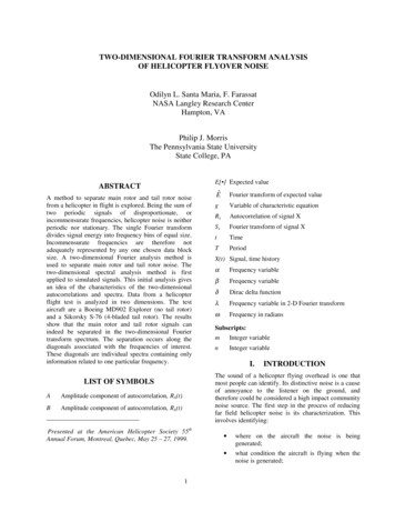
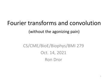
Moreover, as explained in the previous chapter, the quantum Fourier transform can be implementedusing O((log N )2 ) steps. Accordingly, Shor’s algorithm finds a factor of N using an expected numberof roughly (log N )2 (log log N )2 log log log N steps, which is only slightly worse than quadratic in thelength of the input.5.3Shor’s period-finding algorithmNow we will show how Shor’s algorithm finds the period r of the function f , given a “black-box” thatmaps ai 0n i ! ai f (a)i. We can always efficiently pick some q 2 such that N 2 q 2N 2 .Then we can implement the Fourier transform Fq using O((log N )2 ) gates. Let Of denote theunitary that maps ai 0n i 7! ai f (a)i, where the first register consists of qubits, and the secondof n dlog N e qubits. 0i.FqFq. measure. 0iOf 0i.measure 0iFigure 5.1: Shor’s period-finding algorithmShor’s period-finding algorithm is illustrated in Figure 5.1.4 Start with 0 i 0n i. Apply theQFT (or just Hadamard gates) to the first register to build the uniform superpositionq 11 X ai 0n i.pqa 0The second register still consists of zeroes. Now use the “black-box” to compute f (a) in quantumparallel:q 11 X ai f (a)i.pqa 0Observing the second register gives some value f (s), with s r. Let m be the number of elementsof {0, . . . , q 1} that map to the observed value f (s). Because f (a) f (s) i a s mod r, the aof the form a jr s (0 j m) are exactly the a for which f (a) f (s). Thus the first registercollapses to a superposition of si, r si, 2r si, . . . , q r si and the second register collapses4Notice the resemblance of the basic structure (Fourier, f -evaluation, Fourier) with the basic structure of Simon’salgorithm (Hadamard, query, Hadamard).30
to the classical state f (s)i. We can now ignore the second register, and have in the first:m 11 Xp jr si.mj 0Applying the QFT again gives01q 1q 1m 1m1XXjrbsb1 X 1 X 2 i (jr s)b12 i2 i q Aqpe bi pe q @e bi.pqmqmj 0b 0j 0b 0We want to see which bi havesquared amplitudes—those are the b we are likely to see if weP large1 jnow measure. Using that mz (1 z m )/(1 z) for z 6 1 (see Appendix B), we compute:j 0mX1j 0e2 i jrbq mX1 ej 02 i rb jq 8 m:1 e2 i mrbq1 e2 i rbqif e2 i rbqif e2 i rbq 16 1(5.1)Easy case: r divides q. Let us do an easy case first. Suppose r divides q, so the whole period“fits” an integer number of times in the domain {0, . . . , q 1} of f , and m q/r. For the first caseof Eq. (5.1), note that e2 irb/q 1 i rb/q is an integer i b is a multiple of q/r. Such b will havepsquared amplitude equal to (m/ mq)2 m/q 1/r. Since there are exactly r such b, togetherthey have all the amplitude. Thus we are left with a superposition where only the b that are integermultiples of q/r have non-zero amplitude. Observing this final superposition gives some randommultiple b cq/r, with c a random number 0 c r. Thus we get a b such thatbc ,qrwhere b and q are known and c and r are not. There are (r) 2 (r/ log log r) numbers smaller thanr that are coprime to r [48, Theorem 328], so c will be coprime to r with probability (1/ log log r).Accordingly, an expected number of O(log log N ) repetitions of the procedure of this section sufficesto obtain a b cq/r with c coprime to r.5 Once we have such a b, we can obtain r as the denominatorby writing b/q in lowest terms.Hard case: r does not divide q. Because our q is a power of 2, it is actually quite likely thatr does not divide q. However, the same algorithm will still yield with high probability a b whichis close to a multiple of q/r. Note that q/r is no longer an integer, and m bq/rc, possibly 1.All calculations up to and including Eq. (5.1) are still valid. Using 1 ei 2 sin( /2) , we canrewrite the absolute value of the second case of Eq. (5.1) to2 i mrbq 1e 1e2 i rbq sin( mrb/q) . sin( rb/q) The righthand size is the ratio of two sine-functions of b, where the numerator oscillates muchfaster than the denominator because of the additional factor of m. Note that the denominator is5The number of required f -evaluations for period-finding can actually be reduced from O(log log N ) to O(1).31
close to 0 (making the ratio large) i b is close to an integer multiple of q/r. For most of those b,the numerator won’t be close to 0. Hence, roughly speaking, the ratio will be small if b is far froman integer multiple of q/r, and large for most b that are close to a multiple of q/r. Doing thecalculation precisely, one can show that with high probability the measurement yields a b such thatbqc1 .r2qAs in the easy case, b and q are known to us while c and r are unknown.Two distinct fractions, each with denominator N , must be at least 1/N 2 1/q apart.6Therefore c/r is the only fraction with denominator N at distance 1/2q from b/q. Applying aclassical method called “continued-fraction expansion” to b/q efficiently gives us the fraction withdenominator N that is closest to b/q (see the next section). This fraction must be c/r. Again,with good probability c and r will be coprime, in which case writing c/r in lowest terms gives us r.5.4Continued fractionsLet [a0 , a1 , a2 , . . .] (finite or infinite) denotea0 1a1 11a2 .This is called a continued fraction (CF). The ai are the partial quotients. We assume these to bepositive natural numbers ([48, p.131] calls such CF “simple”). [a0 , . . . , an ] is the nth convergent ofthe fraction. [48, Theorem 149 & 157] gives a simple way to compute numerator and denominatorof the nth convergent from the partial quotients:Ifp0 a0 , p1 a1 a0 1, pn an pn 1 pn 2q0 1, q1 a1 ,qn an qn 1 qn 2pnthen [a0 , . . . , an ] . Moreover, this fraction is in lowest terms.qnNote that qn increases at least exponentially with n (qn2qn 2 ). Given a real number x, thefollowing “algorithm” gives a continued fraction expansion of x [48, p.135]:a0 : bxc, x1 : 1/(xa1 : bx1 c, x2 : 1/(xa2 : bx2 c, x3 : 1/(x.a0 )a1 )a2 )Informally, we just take the integer part of the number as the partial quotient and continue with theinverse of the decimal part of the number. The convergents of the CF approximate x as follows [48,Theorem 164 & 171]:If x [a0 , a1 , . . .] then x6 zpn1 2.qnqnConsider two fractions z x/y and z 0 x0 /y 0 with y, y 0 N . If z 6 z 0 then xy 0z 0 (xy 0 x0 y)/yy 0 1/N 2 .32x0 y 1, and hence
Recall that qn increases exponentially with n, so this convergence is quite fast. Moreover, pn /qnprovides the best approximation of x among all fractions with denominator qn [48, Theorem 181]:If n 1, q qn , p/q 6 pn /qn , then xpn xqnp.qExercises1. This exercise is about efficient classical implementation of modular exponentiation.(a) Given n-bit numbers x and N (where n dlog2 N e), compute the whole sequencen 1x0 mod N, x1 mod N , x2 mod N , x4 mod N , x8 mod N ,x16 mod N, . . . , x2mod N ,using O(n2 log(n) log log(n)) steps. Hint: The Schönhage-Strassen algorithm computes the productof two n-bit integers mod N , in O(n log(n) log log(n)) steps.(b) Suppose n-bit number a can be written as a an 1 . . . a1 a0 in binary. Express xa modN as a product of the numbers computed in part (a).(c) Show that you can compute f (a) xa mod N in O(n2 log(n) log log(n)) steps.2. Use Shor’s algorithm to find the period of the function f (a) 7a mod 10, using a Fouriertransform over q 128 elements. Write down all intermediate superpositions of the algorithm.You may assume you’re lucky, meaning the first run of the algorithm already gives a b cq/rwhere c is coprime with r.3. This exercise explains RSA encryption. Suppose Alice wants to allow other people to sendencrypted messages to her, such that she is the only one who can decrypt them. She believesthat factoring an n-bit number can’t be done efficiently (efficient in time polynomial in n).So in particular, she doesn’t believe in quantum computing.Alice chooses two large random prime numbers, p and q, and computes their product N p · q (a typical size is to have N a number of n 1024 bits, which corresponds to bothp and q being numbers of roughly 512 bits). She computes the so-called Euler -function:(N ) (p 1)(q 1); she also chooses an encryption exponent e, which doesn’t share anynontrivial factor with (N ) (i.e., e and (N ) are coprime). Group theory guarantees there isan efficientl
N/2-dimensional Fourier transforms, one of the even-numbered entries of v, and one of the odd-numbered entries of v. This suggest a recursive procedure for computing bv: first separately compute the Fourier trans-form v[even of the N/2-dimensional vector of even-numbered entries of v and the Fourier transform vdodd of