Transcription
TWO-DIMENSIONAL FOURIER TRANSFORM ANALYSISOF HELICOPTER FLYOVER NOISEOdilyn L. Santa Maria, F. FarassatNASA Langley Research CenterHampton, VAPhilip J. MorrisThe Pennsylvania State UniversityState College, PAE[ ] Expected valueABSTRACTA method to separate main rotor and tail rotor noisefrom a helicopter in flight is explored. Being the sum oftwo periodic signals of disproportionate, orincommensurate frequencies, helicopter noise is neitherperiodic nor stationary. The single Fourier transformdivides signal energy into frequency bins of equal size.Incommensurate frequencies are therefore notadequately represented by any one chosen data blocksize. A two-dimensional Fourier analysis method isused to separate main rotor and tail rotor noise. Thetwo-dimensional spectral analysis method is firstapplied to simulated signals. This initial analysis givesan idea of the characteristics of the two-dimensionalautocorrelations and spectra. Data from a helicopterflight test is analyzed in two dimensions. The testaircraft are a Boeing MD902 Explorer (no tail rotor)and a Sikorsky S-76 (4-bladed tail rotor). The resultsshow that the main rotor and tail rotor signals canindeed be separated in the two-dimensional Fouriertransform spectrum. The separation occurs along thediagonals associated with the frequencies of interest.These diagonals are individual spectra containing onlyinformation related to one particular frequency.Amplitude component of autocorrelation, Rx(t)BAmplitude component of autocorrelation, Rx(t)Fourier transform of expected valuegVariable of characteristic equationRxAutocorrelation of signal XSxFourier transform of signal XtTimeTPeriodX(t) Signal, time historyαFrequency variableβFrequency variableδDirac delta functionλFrequency variable in 2-D Fourier transformωFrequency in radiansSubscripts:mInteger variablenInteger variableI.INTRODUCTIONThe sound of a helicopter flying overhead is one thatmost people can identify. Its distinctive noise is a causeof annoyance to the listener on the ground, andtherefore could be considered a high impact communitynoise source. The first step in the process of reducingfar field helicopter noise is its characterization. Thisinvolves identifying:LIST OF SYMBOLSAÊPresented at the American Helicopter Society 55thAnnual Forum, Montreal, Quebec, May 25 – 27, 1999.1 where on the aircraft the noise is beinggenerated; what condition the aircraft is flying when thenoise is generated;
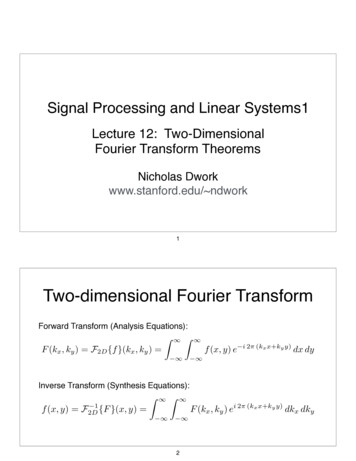
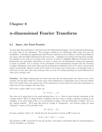
how the noise propagates to the ground.This information can be used to create an illustration orgraphic that visualizes the acoustics of a helicopter. Thegraphic could then be a tool used to identify the areas(flight operations, blade tips, etc) to modify in order toreduce the noise for the listener. The researcher is thuschallenged to create this illustration or graphic thatefficiently conveys the most relevant information.The purpose of this paper is to identify the advantagesof using a 2-D Fourier transform to visualize helicopterflyover noise. Results from this particular 2-D analysiswere first introduced in [1].To explore the possibilities of the 2-D Fouriertransform, this paper will provide the 2-D spectra fromtwo different helicopters: one with a tail rotor, and onewithout. These data, collected during an acoustic flighttest in 1996, will be shown using conventional analysismethods, namely the FFT, as well as with the 2-DFourier transform. The 2-D Fourier transform will beused as an alternate method to distinguish main rotorand tail rotor noise.Some studies have targeted the wakes and tip vorticesshed by the main rotor blades. These wakes and tipvortices not only generate blade-wake interaction andthe highly impulsive blade-vortex interaction noisewhen they encounter other main rotor blades, but theycan also encounter the tail rotor blades and generatemain rotor-tail rotor interaction noise.Noise of the Tail RotorThe tail rotor itself generates the same types of noise asthe main rotor. However, due to its orientation on theaircraft, its surrounding flow field in flight is quitedifferent from that of the main rotor. It is not onlyingesting atmospheric turbulence, it is alsoencountering wakes and vortices from the main rotor,hub, and fuselage. Also, due to its orientation, any noiseradiating in the tail rotor tip path plane would propagateto the ground underneath the tail. References [5], [6],[7], and [8] address tail rotor noise. This type of noisewas observed to be strongest during takeoff for theSikorsky S-76 in Ref. [8].Periodicity of Helicopter NoiseSources of helicopter noiseFigure 1 illustrates the sources of helicopter noise for ahelicopter with a tail rotor. These sources of helicopternoise and their physical meaning are defined in [2].This paper addresses the frequencies associated withmain rotor and tail rotor rotation in the helicopter noisespectrum.Figure 1. Helicopter noise sourcesNoise of the Main RotorAs shown in Fig. 1, the main rotor generates noise inseveral ways: 1) high frequency broadband noise, 2)thickness noise, 3) blade-vortex interaction noise, 4)blade-wake interaction noise, 5) loading noise.Many studies have been conducted to identify, predict,and measure these different sources of main rotor noise.2The main rotor-tail rotor ratio, the multiple of tail rotorrotational frequency in relation to the main rotorrotational frequency, is never designed to be a wholenumber. This prevents the harmonics of the two rotorsfrom reinforcing each other and resonating. Thus thenoise from these two rotors can be characterized as thesum of two periodic signals with incommensuratefrequencies. It is shown theoretically in [4] that thissummed signal is not periodic. Errors described in ref.[9] would result if the 1-D Fourier transform is used ona non-periodic signal. Therefore, Hardin and Miameeproposed in [4] that a 2-D Fourier transform wouldbetter characterize the signal.The following section discusses the 2-D Fouriertransform and explains how it may be used todistinguish main rotor noise from tail rotor noise moreclearly. Section III shows preliminary 2-D Fouriertransform analyses performed on simulated signals toindicate what "ideal" 2-D spectra should look like.Section IV describes the helicopter acoustics flight testfrom which data is analyzed. Section V shows theresults of 2-D Fourier transform analysis on themeasured flyover data, followed by conclusions inSection VI. The advantages of 2-D Fourier transformanalysis on helicopter flyover acoustic data are alsodiscussed in Section VI.
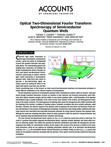
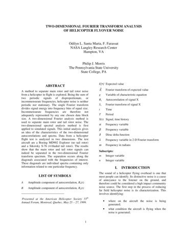
II. 2-D FOURIER TRANSFORMThe 2-D Fourier transform is defined in ref. [10] asS x (λ1 , λ 2 ) R (t , t )e1x j (λ1t1 λ2 t 2 )2dt1 dt 2(1) Rx(t1,t2) is the 2-D autocorrelation of a signal X(t),Rx (t1 , t 2 ) E[X (t1 )X (t 2 )]amplitudes of the diagonals illustrated in Fig. 2 areproducts of different combinations of Am, An, Bm, andBn. These amplitudes along the main or center diagonalwould be for the case m n. It is then possible fromthese center diagonal amplitudes to break down thedifferent components of the amplitude of the paralleldiagonals. This field of amplitude components will notbe applied to the data in this paper. It is simplyintroduced as a subject for further study.(2)E[] is the expected value.In ref. [4], Hardin and Miamee first introduced the 2-DFourier transform as a possible method to separate mainrotor and tail rotor noise. Miamee and Smith [11]developed an estimation of the 2-D spectrum based onthe 1-D spectrum. Although this previous work resultedin an increased understanding of the characteristics e frequencies was not achieved.The estimation of the 2-D spectrum used in this paper isbased on the 2-D autocorrelation shown in Eq. 2.Rx(t1,t2) is calculated using a single sample from a givensignal. The 2-D Fourier transform is then calculatedusing the FFT2 function in the Signal ProcessingToolbox of MATLAB. Estimation of the 2-D spectrumfrom the 2-D autocorrelation resulted in higher tonalresolution than the estimation in [11] which used the 1D spectrum.Ref. [1] provides the derivation of the 2-D Fouriertransform for a signal of the form(4)inω tinω t(X (t ) An e1 Bn e2)nwhere n is the harmonic number, A and B areamplitudes, and ω1 and ω2 are incommensuratefrequencies. The signal X(t) is the sum of periodicsignals with two incommensurate frequencies.The 2-D Fourier transform of X(t) in Eq. 4 is Am Anδ (λ1 nω1 )δ (λ2 mω1 ) An Bmδ (λ1 nω1 )δ (λ2 mω2 ) Eˆ (λ1 , λ2 ) m 1 n 1 Am Bnδ (λ1 nω2 )δ (λ2 mω1 ) Bm Bnδ (λ1 nω2 )δ (λ2 mω2 ) Nwhere(5)Nδ is the Dirac delta function.Figure 2. Support of 2-D power spectral density [4].The next section gives some examples of 2-D Fouriertransform spectra from simulated signals. Theseprovide some idea of the characteristics of 2-D spectraof very simple signals, thus giving a simple preview ofthe expected spectra of real helicopter signals.III. RESULTS WITH SIMULATEDSIGNALSTo get an idea of the expected results from theexperimental data, it is useful to work initially withsimulated or computer-generated data. In the followingsubsections, 2-D spectra are shown for a pure tone, aperiodically correlated signal, and a non-periodicsignal. Since 2-D spectral values are generally complex,the amplitude of the spectra is shown.All calculations are made using a sampling rate of 5000Hz and a rectangular window. To enhance the tonelevels, the sample lengths are multiples of thefundamental frequency of 20 Hz. Multiples of thefundamental frequency at 20 Hz are used for betterresolution.Pure toneFigure 2 shows a schematic of the Dirac delta functionsin the 2-D spectrum, which form a series of diagonallines parallel to the main or center diagonal. The3A simple periodic signal is a sinusoid. Figure 3 showsthe time history and 1-D spectrum of a sinusoidal signal
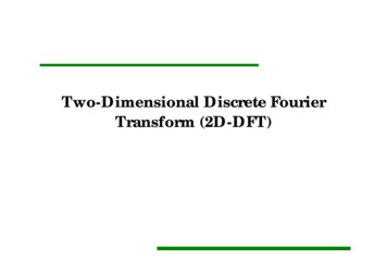
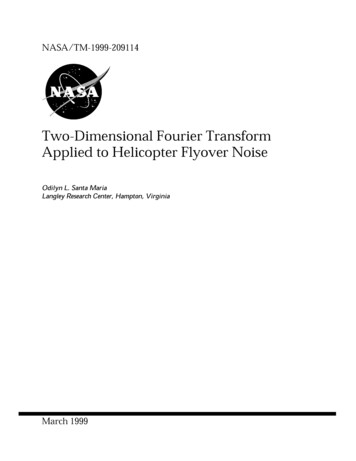
Rxwith frequency 20 Hz. The 1-D spectrum in Fig. 3(b)shows a peak at 20 Hz, as 20.25Time (sec)(a) 2-D autocorrelation(a) Sinusoidal signal, X(t)dB60MAX20 dB S x (f) 40200020406080100120140160180200Frequency (Hz)MIN(b) Spectum, Sx(f) of X(t).Figure 3. Pure tone at 20 Hz, 1-D.(b) 2-D spectrumFigure 4. Pure tone at 20 Hz.The 2-D autocorrelation and 2-D spectrum of the signalshown in Fig. 3(a) are shown in Fig. 4. The diagonal ofthe spectrum in Fig. 4 is equivalent to the single Fouriertransform spectrum that is shown in Fig. 3(c).15105X(t)Periodically Correlated Signal0-5A periodically correlated signal consisting of a puretone and harmonics with decreasing amplitude has alsobeen generated, using MATLAB. For this example, 19harmonics in addition to the fundamental at 20 Hz aregenerated, using the following equation:0.050.100.150.200.25Time (sec)(a) Time history(6)20 dB Sx(f) i 1-150.006020X (t ) (1 .01i ) sin (2π 20it )-1040where t 0 to 409.4 msec in increments of 0.2 msec.Figure 5(a) shows that the time history of the signal upto 0.25 sec has a period of 0.05 sec. Figure 5(b) showsthe 1-D spectrum of the signal, in which all 20 tones(fundamental plus 19 harmonics) can be observed. Thisparticular example resembles the signal from ahelicopter without a tail rotor, such as the MD 902Explorer.Figure 6 shows the 2-D autocorrelation and 2-Dspectrum of the periodically correlated signal. Figure4200100200300400500Frequency (Hz)(b) 1-D SpectrumFigure 5. Periodically correlated signal, 1-D6(a) shows a matrix of dots, which are equally spacedby the period. The "support" lines described in [4] may
be drawn in Fig. 6(b) connecting the intersections of thewhite lines parallel to the diagonal.RxMAXtail rotor tones. The simulated signal includesharmonics with decreasing amplitude for bothsinusoids. The time history of this signal is shown inFig. 7(a). Though it appears periodic in nature, it is infact non-periodic, as explained in the previous section.Figure 7(b) shows the 1-D spectrum of this nonperiodic signal. Note the higher amplitude at 220 Hz,where the 11th and 2nd harmonics, respectively, of thetwo signals are nearly integer multiples of each other.Because their frequencies are so close, the energycontent from both harmonics end up in the samefrequency bins at 110-Hz multiples.25MIN15X(t)(a) 2-D autocorrelation, Rx(t)5-5-15dBMAX-250.000.050.100.150.200.25Time (sec)(a) Time history70 S x (f) 503020 dBMIN100100200300400500Frequency (Hz)(b) 2-D spectrum(b) 1-D SpectrumFigure 6. Periodically correlated signal, 2-D.Figure 7. Periodic signals with incommensuratefrequencies, 1-D.Incommensurate FrequenciesTo simulate a helicopter with a tail rotor, two sinusoidalsignals with incommensurate frequencies are summedusing the following equation:30X (t ) (1 0.01i) sin(2π 20it )(7)i 15( (1 0.01 j ) sin 2π 20 30 jtj 1)where t 0 to 409.4 msec in increments of 0.2 msec.The two frequencies differ by a factor of 30 (20 and20 30 Hz), which approximates the main rotor-tailrotor ratio of the Sikorsky S-76C helicopter. The 20-Hzharmonics will be referred to as the main rotor tonesand the 20 30 ( 110) Hz harmonics will be called the5Figure 8 shows the 2-D autocorrelation and spectrum ofthe simulated non-periodic signal. Close observation ofFig. 8(a) reveals the peaks of the lower (main rotorfrequency) represented as dots, and faint "notches"mark the higher (tail rotor) frequency. Fig. 8(b) showsall the frequencies generated in white, including thehigher (tail rotor) frequency at multiples of 20 and 110Hz.Three diagonals for the center, main rotor, and tail rotorare marked on the 2-D spectrum in Fig. 8(b). The centerdiagonal is equivalent to the 1-D spectrum and containsinformation from all the frequencies in the signal. Themain rotor diagonal, closest to the center diagonal,would only contain information from the main rotorfrequency at 20 Hz. The tail rotor diagonal is parallel tothe center diagonal, offset by 110 Hz, and shouldcontain information only from the tail rotor.
Figure 9shows the center diagonal plotted against themain rotor and tail rotor diagonals. In Fig. 9(a), most ofthe main rotor tones in the main rotor diagonal remainat the same level as in the center diagonal. The first andthird harmonics of the tail rotor at 110 and 330 Hz,respectively, are reduced by over 20 dB in the mainrotor diagonal. The second harmonic of the tail rotor at220 Hz is only reduced by 5 dB, and the fourthharmonic at 440 Hz is reduced by 1 dB. As mentionedabove, the second and fourth harmonics of the tail rotornearly coincide with the 11th and 22nd harmonics of themain rotor. Therefore, it appears that in the main rotordiagonal, the energy in those two frequency bins hasbeen reduced by the contribution of the tail rotor.harmonic of the tail rotor is also shifted one frequencybin lower to 437 Hz in the tail rotor diagonal. There arespikes in the tail rotor diagonal halfway between themain rotor tones that are not present in the centerdiagonal. These minor, or low-level tones represent thediagonal cutting through the white lines seen in Fig.8(b). The major, or high-level tones appear when thediagonal cuts through an intersection of these whitelines. The significance or physical interpretation ofthese minor tones is not explored in this paper."Tail"11595RxMAXdB7555CenterMain20 dB350100200300Frequency (Hz)400500(a) Main rotor diagonal (20 Hz)"Tail"115MIN95dB(a) 2-D autocorrelation75dB55MAXCenter20 dBTail350100200300Frequency (Hz)400500(b) Tail rotor diagonal ( 110 Hz)Figure 9. Diagonals from 2-D spectrum, sum ofincommensurate frequencies.IV. FLIGHT TEST DESCRIPTIONMIN(b) 2-D spectrumFigure 8. Sum of periodic signals with incommensurate frequencies.In Fig. 9(b), most of the main rotor tones are reducedby over 30 dB in the tail rotor diagonal. The first andthird harmonics of the tail rotor retain their centerdiagonal levels, while the second harmonic is reducedby 7 dB, the fourth harmonic by 4 dB. The fourth6The experimental data used in this paper were acquiredduring the 1996 Noise Abatement Flight Test sponsoredby the National Rotorcraft Technology Center (NRTC)and the Rotorcraft Industry Technology Association(RITA). Participating organizations were NASALangley and Ames Research Centers, Volpe NationalTransportation Systems Center (Department ofTransportation), Boeing Mesa, and Sikorsky Aircraft.The test was conducted at the NASA Ames CrowsLanding Flight Test Facility in Crows Landing,California.
The purpose of the test was to validate the DifferentialGlobal Positioning System (DGPS) for precisionguidance for acoustic flight testing, with the specificapplication of designing high precision quieterapproaches. For the purpose of this paper, the flight testparameters provided an extensive database of helicopterflyover noise for main rotor-tail rotor interactionanalysis. Reference [12] describes the purpose andmethodology of the flight test in depth.Test AircraftAmong the aircraft tested were a Boeing MD902Explorer, and a Sikorsky S-76. The Boeing MD902Explorer, shown in Fig. 10, is a five-bladed, eightpassenger helicopter featuring the NOTAR anti-torquesystem (no tail rotor). Its rotor diameter is 33.83 ft, andits maximum takeoff gross weight (MTOGW) is 6250lbs. Reference [13] describes the Boeing Explorerportion of the flight test.which encompassed approximately 1.1 sq. mi. Data wasacquired by four different groups: Sikorsky, BoeingMesa, and Volpe using Sony digital DAT recorders,and NASA Langley using the field digital acquisitionsystem. Microphones labeled N26, N27, and N28 inFig. 12 are used in this paper. These were selected fortheir locations along the flight track, and ease ofaccessing the data. The data from these threemicrophones were recorded on the same tape by one ofthe NASA digital systems. They will be referred to asthe port (N26), centerline (N27), and starboard (N28)microphones hereafter in this paper.Due to the proprietary nature of the acoustic data, noabsolute dB levels are shown in this paper. To allowcomparison of relative levels, scales remain constantbetween microphones in each set of data.Flight ParametersApproaches were flown to a hover over the hover pad,with glideslopes such that the aircraft was at 394 ftaltitude when over the reference microphone. Levelflyovers were flown at various altitudes. For the S-76,departures began at a nominal 200 ft altitude and 394 ftdirectly overhead of the reference microphone. Nodeparture or takeoff data were recorded for the MD 902Explorer.Figure 10. Boeing MD902 Explorer.Figure 11 shows the Sikorsky S-76 test aircraft. It is a4-bladed (44-ft diameter), 10-passenger aircraft with afour-bladed tail rotor (8-ft diameter). Its gross takeoffweight during testing was nominally 11,200 lb, 500 lbless than its MTOGW of 11,700 lb. Reference [14]provides a description and results from the Sikorsky S76 portion of the flight test.Figure 12. Microphone array layout at Crows Landing,CA, during flight test.Data Acquisition and AnalysisFigure 11. Sikorsky S-76.Microphone LayoutThe test aircraft flew over a 50-microphone array laidout on agricultural land adjacent to the Crows Landingmain runway. Figure 12 is a schematic of the array,7Data for the three microphones presented in this paperwere acquired at a 20 kHz sampling rate. Each data runvaried in length, depending on the flight parameterssuch as glideslope, and speed. For the purposes of thispaper, the data used from each flyover were chosenafter inspecting their spectrograms. Spectrograms wereproduced by taking an 8192-point Fast FourierTransform (FFT) every 4096 points of the signal for a
TABLE IAircraft Distances from Microphones50% overlap. Figure 14 is an example of a spectrogramof a flyover.Start Distance (ft) fromEnd Distance (ft) fromFigure 13. Spectrogram of Boeing MD902 Explorerlevel flyover recorded by centerlinemicrophone.The horizontal axis in Fig. 13 denotes time, the verticalaxis denotes frequency, and the sound pressure level(SPL) on a decibel scale is denoted by shade. The mainrotor tones are seen in Fig. 13 as the dark horizontallines beginning at about 40 Hz, and spaced about 40 Hzapart. The Doppler shift is seen as the shift in frequencyof these main rotor tone lines. The frequency shift isespecially severe near the overhead point atapproximately 19 seconds into the flyover. Beyond theoverhead point, some tones at approximately 200 Hzappear as faint gray and white lines at intervals of about180 Hz. These tones are apparently radiated aft of thehelicopter, since they are not very strong prior to theoverhead point. Data segments with high tone levelsand low Doppler shift have been selected as the best torepresent the noise of the flyover.V. RESULTS WITH EXPERIMENTALDATAThe time histories of selected runs from the 1996Crows Landing flight test have been analyzed usingMATLAB software. The first step is to identify, asdescribed in the previous section, a suitable "slice" ofdata from each selected run. A starting point is thenidentified in the signal. From this starting point, asegment with a length of an integer multiple of the mainrotor period is analyzed.Table 1 lists the aircraft distances relative to the threemicrophones used for the start and end of the datasegments used in the Fourier analyses. The last columnof Table 1 shows the distance traveled by the aircraftduring the data set analyzed.8TravelPortCenterStarboardDist. (ft)MD 48S-76Approach328532673287324432263247774541One Dimensional SpectraBoeing MD 902 ExplorerFigure 14 shows the 1-D spectra of a portion of aBoeing MD 902 Explorer level flyover for the threemicrophones specified above. As listed in Table 1, theaircraft was approximately 3200 ft away.The spectra of Fig. 14 show that the noise measured bythese microphones was dominated by the main rotorharmonics. The fundamental BPF tones at 39 Hz for allthree microphones was about 30 dB above the noisefloor. Four harmonics were at least 10 dB above thenoise floor from the port and centerline microphones,and 5 harmonics from the starboard microphone.Disregarding the other discernible tones withcomparatively low sound pressure level (SPL), thesignals whose spectra were shown in Fig. 14 would beconsidered periodic. Therefore, the 1-D spectrumshould be sufficient to describe the noise spectralcharacteristics of this aircraft.Sikorsky S-76 – Level FlightFigure 15 shows the spectra from a Sikorsky S-76 levelflight for the three microphones. As with the BoeingMD 902 Explorer, the Sikorsky S-76 wasapproximately 3200 ft away from the microphonesduring the data segment shown.
1500 ft. As mentioned in Section III, reference [8]indicated a stronger tail rotor signal during takeoff.Indeed, the tail rotor tones are very distinct in thespectra of Fig. 16.110Main Rotor Tones20 dBSPL (dB)9070130Tail Rotor5020 dB110100200300Frequency (Hz)400500SPL (dB)090(a) Port Microphone (Retreating Side)70110Main Rotor Tones5020 dB010090200300Frequency (Hz)400500SPL (dB)(a) Port Microphone (Retreating Side)70130Tail Rotor5020 dB110100200300Frequency (Hz)400500SPL (dB)090(b) Centerline Microphone70110Main Rotor Tones5020 dB0100SPL (dB)90200300Frequency (Hz)400500(b) Centerline Microphone70130Tail Rotor50100200300Frequency (Hz)400500SPL (dB)020 dB11090(c) Starboard Microphone (Advancing Side)Figure 14. Boeing MD902 Explorer spectra for levelflight at 115 knots, 500 ft altitude, 3200 ftuprange of mics.70500The main rotor tones, beginning at 25 Hz, are dominantin the signals from the 3 microphones. The tail rotorfundamental BPF was 141 Hz. Although 10 – 20 dBlower than the highest levels in the three spectra, thetail rotor tones are discernible and are labeled in Fig.15. Note that the tail rotor tone at approximately 280Hz was also a multiple of the main rotor BPF, thereforethere was some energy from the main rotor noise in thisparticular tone.Sikorsky S-76 – TakeoffFigure 16 shows the 1-D spectra from the threemicrophones for a Sikorsky S-76 takeoff. Table 1 liststhe distance from the microphones as approximately9100200300Frequency (Hz)400500(c) Starboard Microphone (Advancing Side)Figure 15. Sikorsky S-76 level flight at 136 knots, 492ft altitude, 3200 ft uprange of mics.Sikorsky S-76 – ApproachFigure 17 shows the 1-D spectra for the threemicrophones for a 6-deg, 74 kt approach of theSikorsky S-76. Helicopter approach noise is typicallydominated by blade-vortex interaction noise (BVI) asthe main rotor blade tip vortices intersect with the mainrotor blades in descent. The three spectra in Fig. 18indeed show sharp peaks for almost every multiple ofthe main rotor BPF up to 500 Hz. These peaks riseapproximately 10 to 20 dB above the noise floor. Thetail rotor BPF can be identified. It can also be observed
Main Rotor100Tail RotorMain Tail20 dB80SPL (dB)that the sound pressure levels are lower for thecenterline microphone, especially at the tail rotorfrequency.60Tail Rotor11020 dBSPL (dB)40900100200300Frequency (Hz)400500(a) Port microphone (retreating side)70501000100200300400500Tail RotorMain Tail20 dBFrequency (Hz)80SPL (dB)(a) Port Microphone (Retreating Side)60Main RotorTail Rotor11020 dB40SPL (dB)090100200300F requency (Hz )400500(b) Centerline microphone70100500100200300400Tail Rotor500Main TailFrequency (Hz)80SPL (dB)(b) Centerline Microphone60Main RotorTail Rotor20 dB1104020 dBSPL (dB)090100200300F requency (Hz )400500(c) Starboard microphone (advancing side)70Figure 17. Sikorsky S-76 6-deg approach at 74 kts,3200 ft uprange of mics.500100200300400500Frequency (Hz)(c) Starboard Microphone (Advancing Side)Figure 16. Sikorsky S-76 takeoff at 74 knots, 1500 ftuprange of mics.Two Dimensional SpectraBoeing MD902 Explorer – Level FlightFigures 18 (a), (b), and (c) show the 2-D spectra fromthe Boeing MD 902 level flight data. These spectraexhibit a similar pattern to the simulated signalspectrum in Fig. 6(b), but with less power in theharmonics above the third.10Diagonals are superimposed on the spectra in Figures18 (a), (b), and (c): one represents the center or maindiagonal of the spectrum, and the other cuts through thefundamental BPF of the main rotor. The centerdiagonals and the fundamental BPF diagonals for thethree microphones are plotted in Fig. 19.The center diagonal of the 2-D spectrum is equivalentto the 1-D Fourier transform of the signal. It containsinformation from all frequencies present in the signal.The main rotor diagonal, in theory, would giveinformation only from the main rotor BPF andharmonics.
110SPL(dB)Center Diag20 dBMain Rotor Diag90SPL (dB)MAX70500100200300400500Frequency (Hz)(a) Port Microphone (Retreating Side)MIN110Center Diag20 dB(a) Power Spectrum, Port MicMain Rotor DiagSPL (dB)9070500100200300400500Frequency (Hz)(b) Centerline Microphone110Center Diag20 dBMain Rotor DiagSPL (dB)9070(b) Power Spectrum, Centerline Mic500dB100200300400500Frequency (Hz)MAX(c) Starboard Microphone (Advancing Side)Figure 19. Boeing MD 902 level flight, center and mainrotor BPF diagonals from 2-D spectra.The main rotor diagonals (solid lines) in Fig. 19 show adecrease in SPL of up to 14 dB for frequencies notassociated with the main rotor BPF. For example, atone around 130 Hz in Fig. 19(b) is reduced by 10 dBfrom the center to the main rotor diagonal. The mainrotor harmonics up to 4 BPF maintained their SPLwithin 4 dB from the center diagonal. Theseobservations indicate that the main rotor diagonalindeed contains mostly information associated with themain rotor BPF. This information could be useful inanalysis of noise generated by the main rotor as itreduces extraneous noise that is included in the overallspectrum.MIN(c) Power Spectrum, Starboard MicFigure 18. Boeing MD902 Explorer 2-D spectra forlevel flight at 115 knots, 500 ft altitude.11
Sikorsky S-76 – Level FlightFigure 20 shows the 2-D autocorrelation and powerdensity spectra for a level flight of the Sikorsky S-76.The autocorrelations and spectra are calculated using ablock length containing ten main rotor periods. Thespectra of Figs. 20 (a), (b), and (c) show higher SPL onthe advancing side of the helicopter rotor.The center, main rotor BPF and tail rotor BPF diagonalsare marked on the spectra of Figs. 20 (a), (b), and (c).The center and main rotor diagonals are plotted togetherin Fig. 21, and the center and tail rotor diagonals areplotted together in Fig. 22.120Center DiagMain Rotor Diag20 dBSPL (dB)SPL (dB)100MAX80600100200300Frequency (Hz)400500(a) Port Microphone (Retreating side)120MINCenter Diag20 dBMain Rotor Diag100SPL (dB)(a) Power Spectrum, Port Mic80SPL (dB)MAX600100200300Frequency (Hz)400500(b) Centerline Microphone120Center Diag20 dBMain Rotor Diag100SPL (dB)MIN80(b) Power Spectrum, Centerline Mic60SPL (dB)0MAX100200300Frequency (Hz)400500(c) Starboard Microphone (Advancing side)Figure 21. Center and main rotor diagonals from 2-Dspectra, Sikorsky S-76 level flight at136 kts.MIN(c) Power Spectrum, Starboard MicFigure 20. Sikorsky S-76 level flight at 136 knots, 492ft altitude.12The main rotor diagonals shown in Fig. 21 show amarked decrease in the SPL at the tail rotor frequencies.This decrease is especially notable in Fig. 21(c), themicrophone located on the advancing side of the rotor,where the tail rotor BPF around 140 Hz decreases byalmost 14 dB. Note that at 2BPF of the tail rotor, thereduction is not as great. This happens to be 11 BPF of
the main rotor, therefore the remaining power should bethe contribution of the main rotor at that frequency.the length of which contains exactly eight periods of themain rotor blade passage. The spectra of Fig. 23 showthe dominant tail rotor peaks, as seen in Fig. 16.120Center Diag20 dBSPL (dB)Tail Rotor DiagMAXSPL (dB)10080600100200300Frequency (Hz)400500(a) Port microphone (Retreating side)MIN120Center Diag20 dB(a) Port Microphone (Retreating Side)Tail Rotor Diag100SPL (dB)SPL (dB)MAX80600100200300Frequency (Hz)400500(b) Centerline microphone
[9] would result if the 1-D Fourier transform is used on a non-periodic signal. Therefore, Hardin and Miamee proposed in [4] that a 2-D Fourier transform would better characterize the signal. The following section discusses the 2-D Fourier transform and explains how it may be used to disting