Transcription
ABSTRACTTitle of Document:DISTRIBUTED TWO-DIMENSIONALFOURIER TRANSFORMS ON DSPs: WITHAPPLICATIONS FOR PHASE RETREIVALJeffrey Scott Smith, Master of Science, 2006Directed By:Professor Bruce JacobDepartment of Electrical EngineeringMany applications of two-dimensional Fourier Transforms require fixedtiming as defined by system specifications. One example is image-based wavefrontsensing. The image-based approach has many benefits, yet it is a computationalintensive solution for adaptive optic correction, where optical adjustments are madein real-time to correct for external (atmospheric turbulence) and internal (stability)aberrations, which cause image degradation.For phase retrieval, a type of image-based wavefront sensing, numerous twodimensional Fast Fourier Transforms (FFTs) are used. To meet the required real-timespecifications, a distributed system is needed, and thus, the 2-D FFT necessitates anall-to-all communication. The 1-D floating point FFT is very efficient on a digitalsignal processor (DSP). For this study, several architectures and analysis of such are
presented which address the all-to-all communication with DSPs. Emphasis of thisresearch is on a 64-node cluster of Analog Devices TigerSharc TS-101 DSPs.
DISTRIBUTED TWO-DIMENSIONAL FOURIER TRANSFORMS ON DSPs:WITH AN APPLICATIONS FOR PHASE RETREIVALByJeffrey Scott SmithThesis submitted to the Faculty of the Graduate School of theUniversity of Maryland, College Park, in partial fulfillmentof the requirements for the degree ofMaster of Science2006Advisory Committee:Professor Bruce Jacob ChairProfessor Shuvra BhattacharyyaProfessor Donald Yeung
Copyright byJeffrey Scott Smith2006
AcknowledgementsThe author would like to thank the Graduate committee for their time andenergies: Bruce Jacob, Shuvra Bhattacharyya, and Donald Yeung.The author would like to thank the NASA Goddard Space Flight Center andthe members of the Optics branch for the support and use of facilities. Thank you andacknowledgements are given to Bruce Dean, David Aronstein, and Ron Shiri for themany useful technical insights and discussions and moral support.Specificappreciation is given to Bruce Dean for his original development and support in theMGS algorithm. The author would like to thank Semion Kizhner and Edward Lo fortheir assistance in the Analog Devices 21160M system, described in Chapter 2. Theauthor thanks Bruce Jacobs, Lee Feinberg, Scott Acton, Peter Maymon, RayBouracut, and Kim Mehalick for discussion and support of this work.The author would like to thank his parents and family; specifically Austinwith his, “How’s Mars?” questions. A special thank you to my girlfriend, Heather,and Mr. Five Stars.ii
ForwardThe author would like to point out the significance of this research. Theresults from this research have become a critical component for NASA, with aspecific application for the James Webb Space Telescope (JWST). The TestbedTelescope (TBT) is a 1/6th scale model of JWST, and is a critical scientific study todemonstrate TRL-6 (Technology Readiness Level) for JWST.1 The results from thisresearch and a working prototype, as described in Chapter 4, are integrated into theTBT.iii
Table of ContentsAcknowledgements .iiForward.iiiTable of Contents .ivList of Tables . vList of Figures .viList of Illustrations .viiiChapter 1 : Introduction. 1Motivation. 1Application. 3Phase Retrieval Algorithm. 6Current Solutions. 11Digital Signal Processors . 13Systems of multiple DSPs. 19Graph Theory . 23Chapter 2 : Phase Retrieval on the ADSP-21160M . 31Algorithm analysis. 31General Optimizations for CPU and DSPs . 34Methodology . 37Results. 38Chapter 3 : Phase Retrieval on the TigerSharc 101 . 41Methodology . 41Computational Precision and Accuracy. 42TS-101: 1, 4, and 8-node . 45TS-101: 16-node architectures . 47TS-101: 16-node architectures analysis. 52TS-101: 32-node and 64-node architecture. 55Chapter 4 : Phase Retrieval on the TigerSharc 201 . 58Hybrid Diversity Algorithm. 58TS-201: 4-node architecture. 59Chapter 5 : Conclusions. 61Summary . 61Future Work . 62Acronyms. 64References and Bibliography . 65iv
List of TablesTbl. 2.1: Timing for 1-D FFT and 2-D FFT for 256 and 512 image size on the21160M.Tbl. 3.1: Scalability for image size on Fig. 3.6.Tbl. 3.2: Timing for various image sizes on three architectures, with 4 DiversityDefocus images after convergence (seconds).v
List of FiguresFig. 1.1: Computation of the 2-D DFT using 1-D FFT building blocks.Fig. 1.2: Various 2-D FFT Libraries: PowerPC 970, single-precision complexinput/output.[2]Fig. 1.3: Wavefront sensing and Control Block Diagram.Fig. 1.4: Block Diagram of focus diversity phase retrieval with two defocus images.[]Fig. 1.5: Block Diagram of MGS using Iterative Transform (ITA) phase-retrieval.Fig. 1.6: Block Diagram of the Analog Devices Sharc 21160M. [20]Fig. 1.7: Block Diagram Analog Devices TigerSharc-TS-101.[20]Fig. 1.8: Block Diagram Analog Devices TigerSharc-TS-201. [20]Fig. 1.9: Block Diagram of 4 Node cluster of ADSP-21160M.Fig. 1.10: Block Diagram of 4 Node cluster of TS-101.Fig. 1.11: Block Diagram of 16 Node cluster of TS-101.Fig. 1.12: Block Diagram of link port connection between cPCI and PMC daughtercard.Fig. 1.13: Block Diagram of 64 Node system of TS-101 with Host Computer.Fig. 1.14: Distributed Transpose on 4 DSPs: Columns represent local memory, andcolors represent data.Fig. 1.15: Two Graphs demonstrating graph diameter: (a) 6 Node Ring, graphdiameter is 3, (b) 8 Node hypercube, graph diameter is 3, distance from N0 to N6is 3, (Node label Nid, d(0,id)).Fig. 1.16: Steps for constructing a graph with minimum diameter: (a) 10 Node basegraph, with 3 edges per node and 6 leaves (b) Peterson Graph: graph diameter is2.Fig. 1.17: Base architectures for several cases: (a) Base architecture for 22 node, 3branches per node, optimal diameter of 3 (b) Base architecture for 17 nodes, 4branches per node, optimal diameter 2 (c) Base architecture of 46 node, 3branches per node, with optimal diameter of 3.Fig. 1.18: Levi graph, 30 nodes and diameter 4. [27]Fig. 2.1: Timing for the phase retrieval algorithm in Matlab: (a) Entire algorithm, (b)details for step 2, with a single iteration.Fig. 2.2: Measured defocus PSF data from the Wavefront Control Testbed (WCT) atGoddard.Fig. 2.3: Phase estimate from the MGS algorithm: (a) Mesh plot, and (b) coloredimage plot.Fig. 2.4: Recovered PSF data from the MGS algorithm.Fig. 2.5: Timing for the phase retrieval algorithm in core iterative algorithm aftermathematical modification.Fig. 2.6: Timing code for 2-D FFTW with and without the second transpose.Fig. 2.7: Optimization of 2-D FFT for padding.Fig. 2.8: Timing for MGS algorithm in Matlab and on the 21160M DSP.Fig. 3.1: Phase estimate after single iteration, Matlab (a), DSP (b), the subtraction ofthe two (c), and the log stretch of the normalized subtraction of the two (d).vi
Fig. 3.2: Phase estimate after algorithm convergence, Matlab (a) the DSP (b), thesubtraction of the two (c), and the log stretch of the normalized subtraction ofthe two (d).Fig. 3.3: Two 8 DSPs grid architectures, hypercube (a) and 1-möbius cube (b).Fig. 3.4: 16 DSP architecture, inefficient use of the PCI bus for all-to-allcommunication.Fig. 3.5: 16 DSP architecture, minimize graph diameter between all 16 DSPs.Fig. 3.6: 16 DSP architecture: minimize graph diameter between clusters.Fig. 3.7: 16 DSP architecture: use PMC cards, and create uni-directional link ports.Fig. 3.8: Four images (a) on 64 DSPs (b) with 16 DSPs per image to produce a singlephase estimate (c).Fig. 3.9: Four images (a) on 16 DSPs (b) with 16 DSPs per image to produce a singlephase estimate (c).Fig. 3.10: 32 DSP Architecture.Fig. 3.11: 64 DSP architecture.Fig. 4.1: Block diagram for the HDA.Fig. 4.2: TS-201 4 DSP architecture.vii
List of IllustrationsIll. 1.1: Segmented primary apertures examples: (a) The Testbed Telescope (TBT) isa 1/6th scale model of the planned James Webb Space Telescope mirror with 18segments in the primary (b) W.M.Keck 1 Observatory with 36 segments in theprimary.[4][5]viii
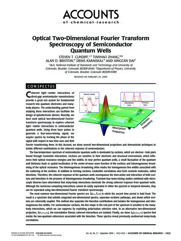
Chapter 1: IntroductionMotivationFor many image-processing algorithms a two-dimensional (2-D) discreteFourier transform (DFT) is required.In all but a few rare cases, the FourierTransform makes use of the Fast Fourier Transform (FFT). The 2-D DFT has amany-to-one mapping, and thus for each element in the output, every element of theinput is required. The 1-D DFT and inverse 1-D DFT can be seen in (Eq. 1.1) and(Eq. 1.2). Similarly, the 2-D DFT and inverse 2-D DFT can be seen in (Eq. 1.3) and(Eq. 1.4) respectively.N "1F [u ] ! f [ x] # e"2# #i#u# xN(Eq. 1.1)xN "1f [ x] ! F [u ] # e2# #i#u# xN(Eq. 1.2)u2 #* #i # x #u")& " 2#* #Ni # y #vN #eF [u , v] ! '' ! f [ x, y ]e y 0 ( x 0%(Eq. 1.3)2#* #i#u# x) N "1& 2#* N#i#v# yN #ef [ x, y ] ! '' ! F [u , v] # e v ( u%(Eq. 1.4)N "1 N "1N "1To compute the 2-D DFT, the function F[u, v] can be constructed by using thebuilding blocks of the 1-D FFT. For this, the 1-D FFT is performed on each row, i.e.compute F[u, y]. Then, the 1-D FFT is performed on column of the result. This isillustrated in Fig. 1.1.1
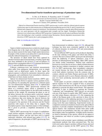
Fig. 1.1: Computation of the 2-D DFT using 1-D FFT building blocks.To access data in column format and row format on a shared memory requiresa transpose of the data. For high-level programming, the transpose of a matrix isstraightforward, i.e. f[x][y] f[y][x]. Yet, for a general-purpose centralprocessing unit (CPU), an efficient transpose is non-trivial due to cache and memoryconstraints. Given a large enough image data size Nsize Nsize, a conventional cachewill not be able to efficiently access both cases of Nsize sequential elements and Nsizeelements that are strided by Nsize. For this reason, the FFT for 2-D has a non-linearperformance with respect to image size on a general purpose CPU, see Fig. 1.2.[2]Specifically, the 2-D FFT sees a significant drop-off with respect to performance forimages of grid size 512 512 or larger. This decrease in performance is in addition tothe performance decrease for the larger image size.2
Fig. 1.2: Various 2-D FFT Libraries: PowerPC 970, single-precision complex input/output.[2]Furthermore, the FFT is optimal in performance for data that is a power oftwo. Yet, for the general purpose CPU, the set associative cache will miss frequentlywhen accessing data that is strided by large powers of two.[3] For this reason, theconfigurable cache is desirable, such as seen in many DSPs, which is already anoptimal choice for a 1-D FFT.ApplicationIn this section, an overview of the optical problem is presented. This justifiesthe motivation for this research without required a deep understanding of the details.Many next-generation scientific optical systems have requirements thatnecessitate adaptive optic control. The use of adaptive optics is an engineering3
technique where optical components are moved in a feedback loop to optimizeperformance. The errors can be internal, such as optical figure error, jitter, andthermal instability or external factors, such as atmospheric turbulence between theobject and the imaging system.These corrections can be made with either adeformable mirror, where the mirror itself is deformable such as a thin membrane, oras a segmented primary mirror, where several rigid-bodied mirrors are piecedtogether to form a large mirror as seen in Ill. 1.1.[4][5] For optical simplicity andefficiency, image-based wavefront sensing is preferable over a conventionalinterferometer-based wavefront sensor.(a)(b)Ill. 1.1: Segmented primary apertures examples: (a) The Testbed Telescope (TBT) is a 1/6th scalemodel of the planned James Webb Space Telescope mirror with 18 segments in the primary (b)W.M.Keck 1 Observatory with 36 segments in the primary.[4][5]For a monochromatic point object that is imaged through an optical system,the light observed in the image plane is called the point spread function (PSF) p(x,y).The PSF is the modulus squared of the coherent system function h(x,y):4
p ( x, y ) h ( x, y )2(Eq. 1.5)The Fourier transform of h(x,y), using (Eq. 1.3) is H(u,v), the coherent systemfunction for the optical system function. The H(u,v) is a complex valued functionrepresented by the pupil function A(u,v) and the phase θ(u,v).H (u , v) A(u , v) " ei"! ( u ,v )(Eq. 1.6)The phase in (Eq. 1.6) is proportional to the optical wavefront. For an idealoptical system, with an optimal PSF, the wavefront is identically zero and thusθ(u,v) 0. For real systems, the wavefront is nonzero and the phase is measured witha wavefront sensor. Then, a correction to the wavefront using the deformable mirrormust be made that induces the negative of the current wavefront, which attempts todrive the system wavefront to zero.[6][7]The fundamental problem is that the wavefront cannot be directly measuredfrom the imaging system. This is because the detector, such as the CCD, observes thePSF. Thus, the phase is lost when the modulus squared is taken, (Eq. 1.5). A simpleway to recognize the problem is to note that only intensity data is known for a Fourierconjugate pair, and it is desire to know the phase data for one or both of the pairs.One solution to the problem is adding additional optics to create an interferometerbased wavefront sensor or a Shack-Hartmann sensor. Both of these solutions havebeen used in practice, but both have known limitations.[8][9][10] Such solutions requirea wavefront reference, introduce non-common path errors, and generally put strongdemands on the number and quality of optical components used.For opticalsimplicity and efficiency, image-based wavefront sensing is preferable over theconventional optical solution. As a result, the image-based approach, while more5
demanding computationally, is generally less complex to implement in hardware andmore attractive from a payload reliability and systems engineering perspective.Although the image-based approach is less complex in hardware than theinterferometer based systems, the increased computational demand h-speeddatatransferandcommunication rates.A block diagram of wavefront sensing and control is shown in Fig. 1.3. It isthe goal of this research to address the specific issue of the computational demand forimage-based wavefront sensing, as outlined as the red block in Fig. 1.3. As a finalnote, it is the science requirements of the optical system that necessitate highprecision optics; and adaptive optics is an engineering tool that provides highprecision optics, without the multi-million dollar cost of high precision optics.Fig. 1.3: Wavefront sensing and Control Block Diagram.Phase Retrieval AlgorithmPhase-retrieval is an image-based wavefront sensing method that utilizespoint-source images (or other known objects) to recover optical phase information.The fundamental component of phase-retrieval is an iterative transform algorithmdeveloped by Misell, Gercherberg, and Saxton; this will algorithm is referred as theMGS.[11][12][13]The NASA Goddard implementation of the MGS is thoroughly6
discussed elsewhere, but will be summarized in this section.[14] The MGS utilizes therelationships between amplitude data in both Fourier domains, and the Fouriertransform relationship that connects the domains.The algorithm estimates the phase !ˆ ( x , y ) in spatial domain and include theknown amplitude data f ( x, y ) in the spatial domain.ˆf1 ( x, y ) f ( x, y ) " e i"! ( x , y )(Eq. 1.7)The algorithm then Fourier transforms to the frequency domain to compute F1 (u , v) .Next, the amplitude data is replaced with the known amplitude data.& F (u , v) #F2 (u , v) F (u , v) ' 1!F(u,v)% 1"(Eq. 1.8)Thus, F2(u,v) has the correct modulus and a phase that is derived from f ( x, y ) . Theinverse Fourier Transform is then computed.& f ( x, y ) #f 3 ( x, y ) f ( x, y ) ' 2!% f 2 ( x, y ) "(Eq. 1.9)The algorithm is repeated until a convergence criteria is meet or a desirednumber of iterations have been executed, at which point, the phase estimate !ˆ ( x , y )is extracted from f n ( x, y ) .With certain data configurations and large array sizes, particularly for undersampled data sets, this core algorithm block can take tens of minutes to several hoursto reach full convergence. This is because two 2-D DFT are required for a single7
iteration of the algorithm. Furthermore, the algorithm may iterate hundreds of timesfor multiple images.It is the goal of this research to document and explore several highperformance computing architectures that capitalize on the limitations ofimplementing this algorithm on a general purpose CPU. As described, the MGS is aniterative algorithm. To speed up the algorithm, there are two techniques that can beutilized. First, the number of iterations can be decreased. Second, the time taken fora single iteration can be decreased. Unfortunately, each iteration of MGS relies onthe answer to the previous iteration, thus the algorithm cannot be implemented inparallel.For the first case, additional techniques have been developed that increase theconvergence rate of the algorithm and thus decrease the number of iterations. Thus,before the algorithm is ported to a distributed high performance computingarchitecture, it is critical to implement and consider all possible ways to increase theperformance of the algorithm. One such technique is called phase diversity. Thedetails of why this helps convergence are beyond the scope of this thesis. Thediversity, ! ( u , v ) , is a known phase term that is added to the H(u,v), such that(Eq. 1.6) becomes:H (u , v) A(u , v) # ei#(" (u ,v ) ! (u ,v ))(Eq. 1.10)Another technique is utilizing of multiple images, where each image has adifferent diversity. Then, each image will produce a phase estimate, and then theindividual phases can be combined (usually a weighted average) into a single estimatefor the system. An example of this technique can be seen in Fig. 1.4. For this block8
diagram, two defocus images are used.The MGS algorithm will produce awavefront. The inverse of the wavefront is then applied to the optical system toremove the estimated aberrations.Fig. 1.4: Block Diagram of focus diversity phase retrieval with two defocus images.[15]The basic MGS algorithm is illustrated in Fig. 1.5. The iterative transformalgorithm (ITA) is the core step that is taken in (Eq. 1.7) through (Eq. 1.9). The MGSrequires numerous iterations from the image plane to the pupil plane via the Fouriertransform pair. For each “inner loop” of MGS and for each image, a single iterationis completed as constraints in each Fourier domain are applied. Thus, a singleiteration results in a Fourier and Inverse Fourier Transform pair; hence, the number of2-D FFTs is the product of the number of diversity-defocus images, the number ofouter loops, the number of inner loops, and a factor of 2 for the Fourier and InverseFourier Transforms of each iteration.9
Fig. 1.5: Block Diagram of MGS using Iterative Transform (ITA) phase-retrieval.An additional technique used for optimization is the appropriate data size.System specifications will necessitate the number of samples in the phase. Foroptimal control, this is the Nyquist sampling relationship to the number of degrees offreedom in deformable mirror or the number of segments. For this application thenumber of samples in the wavefront should be twice the number of degrees offreedom. This aspect of the data size will be fixed by the science requirements, andthus cannot be changed to increase performance. As a system engineering measuringand testing tool, intuitively, more samples in the pupil are desired. There is anadditional optimization with respect to data size. Due to rays of light convergingfrom the pupil to the image plane, the number of samples in both planes are not thesame. Given the number of samples in the pupil plane as defined by the science andoptical requirements, the image plane must have 2 times that amount in both x and ydirections. This is because data is collected in the image plane, and must Nyquistsample the wavefront in the pupil plane. For this reference to the Nyquist samplecriteria, the number of samples in the PSF should be twice the number of samples inthe wavefront in both x and y. Thus, the image plane data has 4 times the number of10
elements as the pupil plane data.This optical relationship allows a furtheroptimization of the MGS because the data reduction will decrease the computationaldemands of the FFT.Current SolutionsCurrent desktop and server line general-purpose central processing units(CPUs) have been optimized for performing multiple tasks and use principles of datalocality to increase performance, yet performance dramatically decreases whenexecuting large 2-D FFTs.[2][3] For example, a current general-purpose CPU can takeseveral seconds for a double precision 2-D FFT of size 2048 2048. This is mainlydue to the fact that the memory architecture is not optimized for such large data sets.To perform the numerous large 2-D FFTs efficiently, several applicationspecific architectures have been developed and are discussed further below. Many1-D and 2-D FFT algorithms exist, yet for each element of the output, the algorithmrequires access to every element of the input.[2][16] Thus, as one naive approach toparallelization, an image cannot be divided into sub-components that are processedcompletely independent. Typically, the 2-D FFT is computed as a series of 1-DFFTs. The total number of 1-D FFTs in the 2-D FFT is then the sum of the number ofthe image size in both rows and columns. For example with the MGS, 4 diversitydefocus images of size 512 512, with 50 outer loops and 10 inner loops result inmore than 4,000,000 1-D FFTs.The process of performing the MGS on Nimg diversity-defocused images ishighly parallel for each image. This is because the weighted average for combing thephases is significantly less computationally demanding than the 2-D FFTs. Recall11
that the data size for the phase is one-fourth the size of the image plane data, and assuch, the communication requirements for the phase averaging routine are smallerthan the communication requirements for the 2-D FFT. Furthermore, a weightedaveraging routine is a ni-to-ni communication problem among the Nnode clusters ofnodes, where only a given node, ni, in a cluster needs to communicate with thecorresponding node in all other clusters.As such, past approaches to increaseperformance have used 1 to Nimg general-purpose CPUs as a cluster.[17]Consequently, this provides a maximum factor of Nimg improvement, while havingthe negative effect of increasing power requirements, footprint, and coolingrequirements by Nimg. The primary solution is to provide Nimg application specific,highly optimized computational cores.All further discussion assumes a singlecomputational core, and thus, the MGS is being performed on a single diversitydefocus image. It should be noted that careful consideration must be made to theinterface between the multiple computational cores, because of the weighted averageof the phase estimates.The computational cores used on each image can be further divided toperform a distributed 2-D FFT.To perform the distributed 2-D FFT, thecomputational requirements scale linearly with the number of sub-components up tothe size of the diversity-defocus image. Thus, the computational requirements of theMGS on a 512 512 diversity-defocus image size scales linearly until one reaches 512sub-components of a computational core, or 512 processing units.Forimplementations of distributed 1-D FFTs, and thus, the scalability for an increase inthe number of sub-components larger than the diversity-defocus image size, various12
algorithms have been explored externally.[18],[19] All discussion in this thesis willassume the 1-D FFT is the smallest component of division.Digital Signal ProcessorsFor this study, three types of digital signal processors were used: AnalogDevices (AD) ADSP-21160M, AD TigerSharc TS-101, and the AD TigerSharcTS-201.[20]Of these three types of DSPs, three systems were constructed ofhomogenous DSP architectures. The first system consists of 8 of the ADSP-21160MDSPs, the second system consists of 64 TS-101 DSPs, and the third system consistedof 24 TS-201 DSPs. The majority of the research in architectural designs was on the64 node TS-101 DSPs. Each of these systems are integrated by Bittware, Inc.It is emphasized that the science requirements necessitate adaptive opticcontrol, and furthermore, the adaptive optics algorithm and performance requirementsnecessitate these types of DSPs. Currently available off the shelf cameras are limitedto 18 bits per pixel or fewer. A naive approach is to set the wavefront sensingalgorithms to this precision. Due to the iterative and feedback nature of the iterativetransform algorithm, errors can quickly propagate. In combination of the desireddynamic range and resolution of the final phase estimate, it can be shown that aminimum of 32-bit float point precision is required for all processing. An example ofwavefront sensing that requires this level of precision is terrestrial planet finding,where the contrast between a star and the planet orbiting around it is 10-9.[21]All of the DSPs in this study have 32 bit floating point precision, with manyother specifications that are characteristic of a modern DSP, including: HarvardMemory Architecture, lower power consumption and a modified instruction set13
architecture (ISA), such as single instruction circular buffer support, single instructionmultiple data (SIMD), and used multiply adds (FMA). It is the lower power ratingthat allows multiple DSPs to exist on a single Peripheral Component Interconnect(PCI) card. The block diagrams of a single 21160M, TS-101, and TS-201 can be seenin, Fig. 1.6, Fig. 1.7, and Fig. 1.8 respectively. Items of significant interest are dualcomputational cores, a link port communication channel, and the direct interconnection between the two.The characteristics of the ISA such as the FMA and the circular buffer supportallow software developers to create a 1-D FFT with the minimal number ofinstructions. Furthermore, because of the SRAM scratch-pad cache, instructions canbe accessed quickly, with a known timing, i.e. there are no cache misses.Furthermore, the circular buffer minimizes the branch miss prediction time. TheSIMD and specifically, the FMA instructions are frequently used in the 1-D FFT.Recall the 1-D FFT in (Eq. 1.1). The 1-D FFT can be divided into two steps bystriding the data of size Nfft, and then performing the 1-D FFT on the even and oddindices of the data, (Eq. 1.11). This division is repeated until Nfft is 2, known asBase-2. Notice how this algorithm is a series of multiplication between the ! n ande"2!# !i!n!kN fft, with a series of sums. If the e"2!# !i!n!kN fftare precompiled as Wn , then the FMAallows the comp
For many image-processing algorithms a two-dimensional (2-D) discrete Fourier transform (DFT) is required. In all but a few rare cases, the Fourier Transform makes use of the Fast Fourier Transform (FFT). The 2-D DFT has a many-to-one mapping, and thus for each eleme