Transcription
Three Dimensional Fast Fourier TransformCUDA ImplementationKumar Aatish, Boyan Zhang
Contents1 Introduction1.1 Discrete Fourier Transform (DFT) . . . . . . . . . . . . . . . . . . . . . .222 Three dimensional FFT Algorithms2.1 Basis . . . . . . . . . . . . . . . . . . . . . . . . . . . . . . . . . . . . . . .2.2 In-Order Decimation in Time FFT . . . . . . . . . . . . . . . . . . . . . .3393 CUDA Implementation113.1 Threadblock Geometry . . . . . . . . . . . . . . . . . . . . . . . . . . . . . 123.2 Twiddle Multiplication . . . . . . . . . . . . . . . . . . . . . . . . . . . . . 153.3 Transpose Kernel . . . . . . . . . . . . . . . . . . . . . . . . . . . . . . . . 164 Experiment Result174.1 Occupancy calculation and analysis . . . . . . . . . . . . . . . . . . . . . . 174.2 Benchmarking . . . . . . . . . . . . . . . . . . . . . . . . . . . . . . . . . . 185 Scope for further improvements5.1 Algorithmic Improvements . . . . . . . . . .5.1.1 CUDA FFT . . . . . . . . . . . . . .5.1.2 Transpose Kernel . . . . . . . . . . .5.2 Kepler Architecture Specific Improvements5.2.1 Register Per Thread . . . . . . . . .5.2.2 Shuffle Instruction . . . . . . . . . .A Occupancy Calculation for Different Thread Block Heights1.1919191920202020
1Introduction1.1Discrete Fourier Transform (DFT)One dimensional Discrete Fourier Transform (DFT) and Inverse Discrete Fourier Transform (IDFT) are given below[Discrete Fourier Transform]:x(k) N 1Xx(n)WNkn , 0 n N 1,(1)n 0x(n) N 11 Xx(n)WN kn , 0 k N 1,N(2)k 0whereWNkn e i2πknN(3)In above discrete transform, the input is N-tuple complex vector x(n), output is vectorwith same length.X Wx(4)If a complex function h(n1 , n2 ) defined over the two-dimensional grid n1 [0, N 1],n2 [0, N 1]. We can define two-dimensional DFT as a complex function H(k1, k2),defined over the same grid.H(k1 , k2 ) NX2 1 N1 1Xe 2πik2 n2 2πik1 n1N2N1h(n1 , n2 )(5)n2 0 n1 0Correspondingly, it is inverse transform can be re-addressed in such form:H(n1 , n2 ) NX2 1 N1 1X 2πik2 n2 2πik1 n11N1e N2h(k1 , k2 )N1 N2(6)k2 0 k1 0Since the Fourier Transform or Discrete Fourier Transform is separable, two dimensionalDFT can be decomposed to two one dimensional DFTs. Thus the computation of twodimensional DFT can achieved by applying one dimensional DFT to all rows of twodimensional complex matrix and then to all columns (or vice versa). Higher dimensionalDFT can be generalized from above process, which hints similar computation solutionalong each transform dimension.[Separability of 2D Fourier Transform]2
2Three dimensional FFT AlgorithmsAs explained in the previous section, a 3 dimensional DFT can be expressed as 3 DFTson a 3 dimensional data along each dimension. Each of these 1 dimensional DFTs can becomputed efficiently owing to the properties of the transform. This class of algorithmsis known as the Fast Fourier Transform (FFT). We introduce the one dimensional FFTalgorithm in this section, which will be used in our GPU implementation.2.1BasisThe DFT of a vector of size N can be rewritten as a sum of two smaller DFTs, each of sizeN/2, operating on the odd and even elements of the vector (Fig 1). This is know as theDanielson-Lancsoz Lemma [G. C. Danielson and C. Lanczos] and is the basis of FFT. .So-called fast fourier transform (FFT) algorithm reduces the complexity to O(N logN ).Danielson-Lancsoz Lemma:N2X(k) 1Xx(2n)e2π (2n)k iNN2 n 0 x(2n 1)e i2π (2n 1)kNn 0N2 1X 1Xx(2n)e i 2πnkN2N2 n 0 1Xx(2n 1)e i 2πnkN2n 0 DF T N [x0 , x1 , . . . , xN 2 ] WNK DF T N [x1 , x3 , . . . , xN 1 ]22If N is a power of 2, this divide and conquer strategy can be used to recursively breakdown the transform of size N into log2 (N ) transforms of length 1 leading to performanceincrease (O(N log2 N )) over a nave matrix multiplication of a vector with the DFT matrix(O(N 2 )).The exact method of decomposing the larger problem into smaller problems can varywidely. A number of algorithms have been proposed over the years, the most famousof which is the Cooley-Tukey Algorithm[Cooley, J. W. and Tukey, O. W.] which has twovariations called the Decimation in Time (DIT) and Decimation in Frequency (DIF).3
Figure 1: Recursive Relation (DIT FFT) : 1. 2 * N/2-radix DFT 2. Twiddle Multiplication 3. N/2 * 2-radix DFTs[Decimation-in-time (DIT) Radix-2 FFT]In the DIT FFT (Fig 1) , if a vector is of size N N1*N2, the DFT formulation isdone by:4
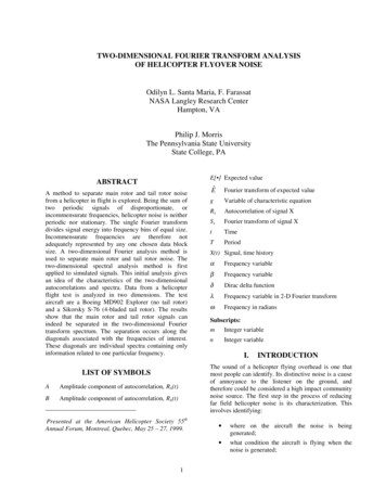
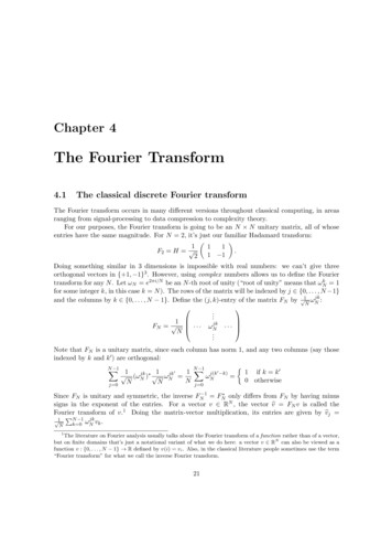
Figure 2: Recursive Relation (DIF FFT) : 1. N/2 * 2-radix DFTs 2. Twiddle Multiplication 3. 2 * N/2-radix DFT[Decimation-in-time (DIT) Radix-2 FFT] Performing N1 DFTs of size N2 called Radix N2 FFT. Multiplication by complex roots of unity called twiddle factors. Performing N2 DFTs of size N1 called Radix N1 FFT.The DIF FFT, the DFT formulation is: Performing N2 DFTs of size N1 called Radix N1 FFT. Multiplication by complex roots of unity called twiddle factors. Performing N1 DFTs of size N2 called Radix N2 FFT.In this paper, we implement the DIT FFT for length 128, although, according to ourhypothesis, an equivalent DIF FFT would not differ in performance. By using this 1285
element FFT, we can further construct FFT algorithms for different sizes by utilizingthe recursive property of FFTs. However, such an exercise is not under the scope of ourproject.In the DIT scheme, we apply 2 FFT each of size N/2 which can be further brokendown into more FFTs recursively. After applying each such recursive relation, we get acomputation structure which is popularly referred to as a Butterfly.W (N,N) 12(7)Therefore, W (N, k) can be expressed as W (N, k N N), k N 12 2(8)Since we can express half of the twiddle factors in terms of the other half, we haveN2 twiddle multiplication at each stage, excluding multiplications by -1. For an input(G(i), H(i)) the function B(G(i), H(i)) (G WNi H(i), G WNi H(i)).Figure 3: Butterfly [Signal Flow Graphs of Cooley-Tukey FFTs]It should be noted that while breaking down the FFT of size N into two FFTs of sizethe even and odd inputs are mapped out of order to the output. Decomposing thisproblem further to FFTs of the smallest size possible would lead to an interesting orderof input corresponding to the output. Upon inspection, we can see (Fig 4) that an inputhaving an index k, had a corresponding output with index as bitreverse (k, log2 (N )), i.e.the bit reversal done in log2 (N ) bits.N2,6
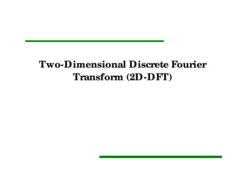
Figure4:Radix-2DITFFT[Decimation-in-time (DIT) Radix-2 is pattern can be explained by the fact that applying an FFT of length N2 wouldrequire reshuffle of input indices into even odd relative to the new transform lengthafter the decomposition, e.g. N2 after the first decomposition. This would be the same as7
sorting with length (2pN 1) with respect to the p 1th bit first and then by the remainingbits in the pth 101111100010001011000110101111101234567After the complete decomposition of the problem is achieved, we would be left with anFFT of length 2 and the number of decompositions done would be log2 (N ). Thus wecan do the FFT in log2 (N ) time steps, and each such step is referred to as Stages in thispaper.8
2.2In-Order Decimation in Time FFTA DIT FFT does not necessarily imply an out of order input and an in order output.We can reshuffle the input order at the expense of ordering of the output. For example,in Fig 5, for the case of FFT length 16, the reshuffled butterfly diagram has inorder input and out-of-order output. For the development of our GPU algorithm, thisapproach would be more conducive for coalesced memory access.As mentioned before, it is easy to observe that after every stage, there are alwaysN2 twiddle multiplications. This is due to the fact that every decomposition stage p,there are 2Np twiddle factors introduced by 2p 1 DFTs. As the recursive relation leadsto smaller transform lengths, the range of twiddle factors introduced at each step varies.It is because of this reason that the difference between a DIT and DIF implementationof FFT is the range of twiddle factors W Q used to multiply the intermediate valueswith before every stage. Fortunately, the values that the twiddle factors take can bedetermined, although the relationship between the twiddle factors and the input indexis not so obvious.9
Figure 5: DIT FFT, In-order input, out-of-order output. Every stage has N/2 twiddlefactors [Decimation-in-time (DIT) Radix-2 FFT]Stagekinput indexrange(Q)1230-3, 4-70-1, 2-3, 4-5, 6-70, 1, 2, 3, 4, 5, 6, 74-7, 12-152-3, 6-7, 10-11, 14-151, 3, 5, 7, 9, 11, 13, 15040, 4, 2, 60, 4, 2, 6, 1, 5, 3, 7At every stage, the Stride is defined to be (2Np ) and each such stage consists of 2p 1sets of butterflies. Depending upon whether the input element index falls on the lowerhalf or the upper half of a butterfly set, elements are either added to or subtracted10
from elements across a stride. More precisely, the following pseudocode demonstrate theADDSUB step of each stage:i f ( ( t i d & STRIDE( p ) ) STRIDE( p ) ){v a l [ i ] v a l [ i STRIDE( p ) ] v a l [ i ] ;}else{v a l [ i ] v a l [ i STRIDE( p ) ] v a l [ i ] ;}After the ADDSUB step, the MUL TWIDDLE step takes place for all stages except thelast onei f ( ( t i d & STRIDE( p 1)) STRIDE( p 1)){v a l [ i ] v a l [ i ] TWIDDLE KERNEL( i , p , N ) ;}Our implementation, does not make function calls to generate twiddle factors but areinstead hard coded. A general relation between the kth twiddle factor and its value Q canbe expressed as bitreverse(F LOOR[k/(N/2p )], log2 (N ) 1).[Computing FFT Twiddle Factors]This idea has been applied to our implemented case of length 128 and a detailedrelation between input index and Q is given in the next section.3CUDA ImplementationOur implementation does an FFT transform in the row major dimension of a given threedimensional matrix at a time. Thus, the complete 3D FFT is a set of 1D FFT kernelsand transpose kernels which bring a desired coordinate axis to the row major formatto enable coalesced global reads. The implemented kernel performs a single precision1D FFT and uses the fast math functions for calculating the sin and cos of the phasescorresponding to twiddle factors.The GPU used is the C2050 Fermi GPU on the DIRAC cluster on the Carver systemprovided by the National Energy Research Scientific Computing Center. The NVIDIATesla C2050 has 448 parallel CUDA processor cores with 3 GB of memory.11
3.1Threadblock GeometryThe threadblock geometry and global data mapping onto the block can be done in moreways than one.Figure 6: Serial Configuration of thread block mapping(Fig 6) shows that each CUDA thread within a thread block manages entire rowvector transform. this configuration does not meet memory usage requirement for largeinput data size because of limitation of local storage space (registers per thread). Moreover, reads from global memory are not coalesced.12
Figure 7: Serial Configuration of thread block mapping(Fig 7) shows a different mapping approach of thread block structure. Threads withinone thread block are working on a single row vector. Required communication amongdifferent threads only happens within each thread block.13
Figure 8: Serial Configuration of thread block mapping(Fig 8) is a modified configuration for that showed in (Fig 7)., a single row of threadsare grouped within one thread block responsible for calculating the transform of morethan one row of data. If we assume length of transform vector is 128, upto 4 rows canbe grouped within one thread block. For the optimal number, a trade-off may be madebetween multiprocessor computing ability and resource.We have implemented the third alternative that transforms more than one row ofdata by a single row of threads resulting in higher Instruction Level Parallelism. Eachsuch threadblock is assigned a shared memory block of height H and row size TLEN 128. Since, we are dealing with complex numbers two identical shared memory blocksare maintained for both real and imaginary components of the data.The real and imaginary component of the data is loaded onto the shared memoryfrom the global and is also read into the registers. After this step each of the 7 stagesof the FFT are computed. Each of these stages consists of the ADDSUB step, that is,every thread reading data element of a thread either STRIDE(p) ahead and add thevalue to its own value, or read from a thread STRIDE(p) behind and subtract its ownvalue from this value.The next stride value STRIDE(p 1) decides which of these elements get multipliedby the twiddle factor. Those threads that satisfy the condition are allowed to multiply14
their data with the twiddle factor, after which the resultant data is written back to theshared memory to be used by the threadblock. This sequence of steps continues till theFFT is completed. The last stage however, does not involve multiplication by twiddlefactor and only consists of the ADDSUB step after which the values of each thread is firstwritten to the bit reversed column in the shared memory. The data is then read backto the registers of every thread in a contiguous pattern and then written to the globalmemory in a coalesced fashion. Although an increased H would apparently increasethe instruction level parallelism there are limits to the range of H as it can cause loweroccupancy due to limitation of shared memory resource. Apart from shared memory, anincreased H would also cause an increased register pressure and could lead to registerspilling leading to inefficient execution and lowered performance. Even if we somehowlimit the row size so that H * TLEN is lesser than 32 KB (Available register memory), asevere limitation of the Fermi architecture is that it only allows 63 registers per thread.Due to these concerns, we experimentally determined the optimal height H for whichthe 1D FFT kernel would be most efficient. These experiments are dealt with in theExperimental Results section.3.2Twiddle MultiplicationAs explained in the Algorithms section, the relationship between the kth twiddle factorand the twiddle factor value Q is given by bitreverse(F LOOR[k/(N/2p )], log2 (N ) 1).Since our implementation maps elements of the transformed vector along the threadblock, the thread index maps directly to the input index.For our case, N 128, log2 (N ) 1 6 For p 1,Figure 9: Twiddle factors for stage 1For p 2,15
Figure 10: Twiddle factors for stage 2A general pattern emerges from these two tables. For any given thread id in the pthstage, the most significant p bits are reversed in log2 (N ) 1 bits and remaining bitsare ignored. For e.g., for stage 5, if the thread id corresponding to a particular dataitem, which is to be multiplied with a twiddle factor is of the type ABCDEXY, then thevalue of Q, which is to be multiplied with the data item, is EDCBA0. For each of thestages for N 128, different bit reversal techniques were used to maximize performance.More often that not, unnecessary operations were removed from a generalized 6 bit, bitreversal.3.3Transpose KernelOur 1D FFT kernel is designed to work in the row major dimension. Due to this, afterperforming a 1D FFT, we must transpose the global data so that the 1D FFT kernel canwork in a different data dimension. Since the 3D FFT would also encompass transposeoperations, it is imperative that an efficient transpose kernel is developed. CUDA SDKprovides a great example for starting with two dimensional square matrix transpose[Optimizing Matrix Transpose in CUDA]. The optimized kernel removes uncoalescedmemory accessing and shared memory bank conflicts. We modified transpose kernel toadapt to our requirement for three dimensional transpose.Considering the stride between sequence elements is large, performance tends todegrade for higher dimensions. Global transpose is involved with significant amountof global memory operation, consequently, optimized transpose operation is critical forachieving better overall performance. Before performing the 1D FFT, the data dimensionin which the transform is desired is brought down to the lowest dimension. After thisprocess is completed for all the data dimensions, the data is transposed back to theoriginal data dimensions. In totality, the 1D FFT kernel is called thrice interspersedwith 4 transpose kernels.16
44.1Experiment ResultOccupancy calculation and analysisAppendix A lists figures result of occupancy testing for multiprocessor warp occupancyunder different thread block height configurations. It can be shown that when H 16, local shared memory usage serves as limiting factor for warp occupancy rate. Eachthread block is assigned 16KB shared memory block. On Dirac GPUs with 2.0 computecapability [Node and GPU Configuration], each multiprocessor has only 48KB sharedmemory space available. Applying this calculation to the case when H 8, we foundthat the concurrent executing threadblock on each multiprocessor is 6 which is less thanphysical limits for active thread block. The optimal height H is 4, although it delivers same occupancy rate with smaller height size, but better local memory bandwidthutilization benefits memory accessing latency hiding. However, occupancy calculationalso shows possibility for further improvement, each threadblock can have more threadswithout touching/reaching register and shared memory usage critical points. Based ondiscussion above, we expect implementation scheme such as assigning 2xTLEN threadsfor one thread block will deliver better performance, although without implementationand test result to support the hypothesis.Figure 11: FFT 1D Implementation Vs. CUFFT 1D17
Figure 12: FFT 1D Implementation Vs. CUFFT 3DFigure 13: FFT 3D Execution Time (ms)4.2BenchmarkingTwo testing schemes are utilized for benchmarking our kernel with CUFFT library performance. 1D CUFFT plan (1D in place transform) over three dimensional data18
3D CUFFT plan (3D in place transform) over three dimensional data5Scope for further improvements5.15.1.1Algorithmic ImprovementsCUDA FFTThe algorithm employed in this project can be improved further by utilizing registermemory for FFT transform. Recall that the optimum height of a global data chunkbelonging to a thread block is 4. Before starting a 1D FFT along the row major direction,suppose in a thread block every thread having global Y index tid y were to load the datarow with index bitreverse(tid y). This would be followed by a 1D FFT in the row majordirection. Since the Height is 4, every thread has 4 elements in the Y direction, but sincewe have loaded rows corresponding to bitreverse(tid y), , each thread would be able tofinish the first two stages of the FFT in the Y direction using register memory withoutsynchronization getting into the picture. This would be followed by 2 transposes so thatthe Y data dimension becomes row major and Z data dimension becomes column major,however its indices would be bitreversed. This would be followed by 1D FFT in therow major order. Since we have read the rows in the bitreverse order in the last 1DFFT, currently, the input to the 1D FFT would be out of order, the data would alreadybe in the third stage of the 1D FFT computation and the final output data would bein-order. This would be followed by the same sequence of instructions till the 3D FFTis computed.5.1.2Transpose KernelCurrent implementation of the 3D FFT involves calls to two transpose kernels after thethird 1D FFT is completed. These two calls individually exchange the data dimensionsXY and YZ to undo the effect of transpose required by the 1D FFT kernels. It is possibleto merge these two transpose kernels to transpose X, Y and Z dimensions simultaneously.Since each transpose kernel spends non-trivial time calculating its new index, instructionlevel parallelism can be utilized to hide the memory latency.19
5.2Kepler Architecture Specific Improvements5.2.1Register Per ThreadOne of the prime reasons why the Height of data chunk assigned to a thread block couldnot be increased is due to register pressure. It would be possible to increase this Heightin Kepler GK110 since the maximum number of registers per thread possible has beenraised to 255 as compared to 63 in Fermi. An increased Height could mean an improvedperformance since it would allow even more stages of computation of column majorFFT (as explained in the previous subsection) to be computed by a single thread usingregister memory only.5.2.2Shuffle InstructionIt is quite possible that the shared memory usage of the 1D FFT Kernel be drasticallyreduced because of the shuffle instruction. Shuffle Instruction enables data exchangewithin threads of a warp, hence shared memory usage would go down as a result. Forout of order input and in-order output, this would be especially more beneficial becausethe first few stages would eliminated the need for inter warp communication.AOccupancy Calculation for Different Thread Block HeightsH 120
Figure 14: Threads Per Block Vs. SM Warp OccupancyFigure 15: Registers Per Thread Vs. SM Warp Occupancy21
Figure 16: Shared Memory Usage Vs. SM Warp OccupancyH 2Figure 17: Threads Per Block Vs. SM Warp Occupancy22
Figure 18: Registers Per Block Vs. SM Warp OccupancyFigure 19: Shared Memory Usage Vs. SM Warp Occupancy23
H 4Figure 20: Threads Per Block Vs. SM Warp Occupancy24
Figure 21: Registers Per Block Vs. SM Warp OccupancyH 825
Figure 22: Threads Per Block Vs. SM Warp OccupancyFigure 23: Registers Per Block Vs. SM Warp Occupancy26
Figure 24: Shared Memory Usage Vs. SM Warp OccupancyH 1627
Figure 25: Threads Per Block Vs. SM Warp OccupancyFigure 26: Registers Per Block Vs. SM Warp Occupancy28
References[Discrete Fourier Transform] http://en.wikipedia.org/wiki/Discrete Fourier transform[Separability of 2D Fourier Transform] www.cs.unm.edu/ williams/cs530/ft2d.pdf[The Cooley-Tukey Fast Fourier Transform Algorithm] http://cnx.org/content/m16334/latest/#uid8[Node and GPU Configuration] rac/node-and-gpu-configuration/[Optimizing Matrix Transpose in CUDA][G. C. Danielson and C. Lanczos] ”Some improvements in practical Fourier analysis andtheir application to X-ray scattering from liquids”, J. Franklin Inst. 233, 365 (1942)[Cooley, J. W. and Tukey, O. W.] ”An Algorithm for the Machine Calculation of Complex Fourier Series.” Math. Comput. 19, 297-301, 1965.[Computing FFT Twiddle Factors] mation-in-time (DIT) Radix-2 FFT] http://cnx.org/content/m12016/latest/[Signal Flow Graphs of Cooley-Tukey FFTs] http://cnx.org/content/m16352/latest/29
2) (6) Since the Fourier Transform or Discrete Fourier Transform is separable, two dimensional DFT can be decomposed to two one dimensional DFTs. Thus the computation of two dimensional DFT can achieved by applying one dimensional DFT to all rows of two dimensional complex matrix and then to all col