Transcription
Ellipsometry in Interface ScienceH. Motschmann and R. TeppnerMax-Planck-Institut für Grenzflächenforschung, GolmContents1 What is it all about?22 Polarized light23 Basic equation of ellipsometry54 Design of an ellipsometer65 Theory of reflection106 Ellipsometry applied to ultrathin films177 Microscopic model for reflection198 Adsorption layers of soluble surfactants238.1Importance of purification . . . . . . . . . . . . . . . . . . . . . . . . . . .238.2Physicochemical properties of our model systems. . . . . . . . . . . . . .238.3Adsorption layer of a nonionic surfactant . . . . . . . . . . . . . . . . . . .248.4Ionic surfactant at the air-water interface . . . . . . . . . . . . . . . . . . .258.5Kinetics of absorption . . . . . . . . . . . . . . . . . . . . . . . . . . . . .349 Principle of imaging ellipsometry369.1Depth of field problem . . . . . . . . . . . . . . . . . . . . . . . . . . . . .379.2Beyond the diffraction limit . . . . . . . . . . . . . . . . . . . . . . . . . .39
21What is it all about?The following chapter presents the basics of ellipsometry and discusses some recent advances. The article covers the formalism and theory used for data analysis as well asinstrumentation. The treatment is also designed to familiarize newcomers to this field.The experimental focus is on adsorption layers at the air-water and oil-water interface.Selected examples are discussed to illustrate the potential as well as the limits of thistechnique. The authors hope, that this article contributes to a wider use of this techniquein the colloidal physics and chemistry community. Many problems in our field of sciencecan be tackled with this technique.Ellipsometry refers to a class of optical experiments which measure changes in the stateof polarization upon reflection or transmission on the sample of interest. It is a powerfultechnique for the characterization of thin films and surfaces. In favorable cases thicknessesof thin films can be measured to within Å accuracy, furthermore it is possible to quantifysubmonolayer surface coverages with a resolution down to 1/100 of a monolayer or tomeasure the orientation adopted by the molecules on mesoscopic length scales. The highsensitivity is remarkable if one considers that the wavelength of the probing light is onthe order of 500 nm. The data accumulation is fast and allows to monitor the kinetics ofadsorption processes. The technique can also be extended to a microscopy. Imaging ellipsometry allows under certain conditions a direct visualization of surface inhomogeneitiesas well as quantification of the images. Many samples are suitable for ellipsometry andthe only requirement is that they must reflect laser light. Its simplicity and power makesellipsometry an ideal surface analytical tool for many objects in interface science.2Polarized lightLight is an electromagnetic wave and all its features relevant for ellipsometry can bedescribed within the framework of Maxwell’s theory [1]. The relevant material propertiesare described by the complex dielectric function or alternatively by the correspondingrefractive index n.
3 and a magnetic field B. The fieldAn electromagnetic wave consists of an electric field Evectors are mutually perpendicular and also perpendicular to the propagation directionas given by the wave vector k. All states of polarization are classified according to thetrace of the electrical field vector during one period. Linearly polarized light means theelectrical field vector oscillates within a plane, elliptically polarized light means that thetrace of the electric field vector during one period is an ellipse. A convenient mathematicalrepresentation of a given state of polarization is based on a superposition of two linearlypolarized light waves within an arbitrarily chosen orthogonal coordinate system. E cos(2πνt k · r δp ) r, t) p E( Es cos(2πνt k · r δs )(1) Ep and Es are the amplitudes, δp and δs the phases, k 2π/λ is the magnitude of thewave vector and ν the frequency. Only the phases δp , δs and the amplitudes are requiredfor a representation of the state of polarization; the time dependence is not of importanceand can be neglected. The so called Jones vector reads E Es e Ep eiδpEp iδsEs (2)Different states of polarization are depicted in Fig. 1. The state of polarization isa) linear, if δp δs 0 or δp δs π,b) elliptical, if δp 6 δs and Ep 6 Es ,c) circular for the special case δp δs π/2 and Ep Es .Phase dlefthandedFigure 1: The Jones representation of polarized light represents any state of polarization as a linearcombination of two orthogonal linearly polarized light waves.
4An alternative representation of a given state of polarization uses the quantities ellipticityω and azimuth α. The ellipticity is defined as the ratio of the length of the semi-minoraxis to that of the semi-major axis as shown in Fig. 2. The azimuth angle α is measuredcounterclockwise from the xÝ-axis. Light is assumed to propagate in positive zÝ directionso that xÝ, yÝ and zÝ define a right handed coordinate system. Some authors prefer thisrepresentation and for this reason the conversion formulas between both notations arelisted below. The derivations require a vast number of tedious algebraic manipulationsand can be found in [2].2Ex Ey cos(δy δx ) 90 α 90 Ex2 Ey22Ex Ey sin(δy δx )sin(2ω) 45 ω 45 Ex2 Ey2tan(2ω) 180 δy δx 180 tan(δy δx ) sin(2α)²² ³³Eycos 2 arctan cos(2ω) cos(2α)0 arctan(Ex /Ey ) 90 Extan 2α (3)(4)(5)(6)Ambiguities arising from the inversion of trigonometric functions are settled if the upperand lower limits of all quantities are considered.Figure 2: Elliptically polarized light defined by the azimuth α and the ellipticity ω
53Basic equation of ellipsometryA typical ellipsometric experiment is depicted in Fig. 3. Light with a well defined stateof polarization is incident on a sample. The reflected light usually differs in its state ofpolarization and these changes are measured and quantified in an ellipsometric experiment.PpsoSFigure 3: Ellipsometric experiment in reflection modeThe mathematical description is best done within the laboratory frame of reference definedby the plane of incidence. The propagation direction of the beam and the normal of thereflecting surface define the plane of incidence. Light with an electric field vector oscillatingwithin the plane of incidence (Ýp-light) remains linearly polarized upon reflection and the perpendicular to the plane of incidence. For this reason pÝsame holds for sÝ-light with Eand sÝ-light are also called Eigen-polarizations of isotropic media or uniaxial perpendicularmedia. This consideration makes it obvious that this frame of reference is distinct. Incidentand reflected beam can be described by their corresponding Jones vector : r iδpri iδpi Ep e Ep e inc refl EE ir Esi eiδs Esr eiδsTwo quantities Ψ(7)and are introduced in order to describe the changes in the state ofpolarization. (δpr δsr ) (δpi δsi )(8)
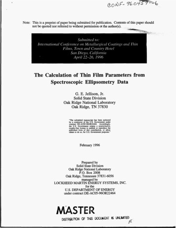
6tan Ψ Epr / Epi r Es / Esi (9)Changes in the ratio of the amplitudes are described as the tangent of the angle Ψ . It willturn out later that Ψcan be directly measured.The reflectivity properties of a sample within a given experiment are given by the corresponding reflection coefficients rp and rs . The reflection coefficient is a complex quantitythat accounts for changes in phase and amplitude of the reflected electric field E r withrespect to the incident one E i .rp Epr i(δr δi )e p p Epi rs Esr i(δsr δsi )e Esi (10)Interference cannot be observed between orthogonal beams and hence pÝ- and sÝ-light donot influence each other and can be separately treated. With these definitions the basicequation of ellipsometry is obtainedtan Ψ · ei Eqn. (11) relates the quantities Ψrp ρ (ρ) i (ρ)rs(11)and with the reflectivity properties of the sample.The following two section discuss various ways to measure and Ψand the theory andalgorithm used for a calculation of the complex reflectivity coefficient. Some ellipsometersare designed in a way that they measure directly the real and imaginary part of the complexquantity ρ instead of Ψ4and . Eqn. (11) allows a conversion between both notations.Design of an ellipsometerMany different designs of ellipsometers have been suggested and a good overview is presented in Azzam and Bashara [3]. Here we discuss common roots of all arrangements andthe underlying theory.The layout of a typical ellipsometer is depicted in Fig. 4. The main components are apolarizer P which produces linearly polarized light, a compensator C which introduces adefined phase retardation of one field component with respect to the orthogonal one, thesample S, the analyzer A and a detector.
7Laser rSampleFigure 4: Ellipsometer in a PCSA-configurationThis setup allows the determination of the unknown ellipsometric angles and can be operated in various modes. Each optical component modifies the state of polarization. Sinceany state of polarization can be represented by a complex Jones vector consisting of twocolumns, the effect of each optical components is described by a complex 2 2 matrix.The Jones formalism provides an elegant means for a quantitative description [4]. ExEy Ja T11 T12T21 T22 J ExEy Je Je TJ E(12)The superscript J refers to the optical component J [PCSA]; the subscripts e and a refer to the E-vectorbefore and after the component. Each of the optical componentsincluding the sample possesses a distinct coordinate system in which the correspondingmatrix is diagonal. For example a compensator consist of a birefringent material cut to athin plate of a defined thickness t. Optically it possesses a fast and a slow axis. Linearlypolarized light oscillating parallel to either axis remains linearly polarized, however, sincethe corresponding refractive indices of fast nf and slow axis ns differ, they travel withdifferent speed which leads to a phase shift φ (nf ns ) · t · 2π/λ between the twocomponents. Similar expressions can be given for each component:
8componentPolarizerCompensatorcoordinate systemJones-Matrix tP transmission axisTP eP extinction axis sc slow axisTC lc fast axiswithρc tc eiδc psAnalyzer 00 1 0 0 ρc rp 0 EsCa i(δs δl )e ElCa eigenpolarizationSample10 TS parallel to plane of incidenceperpendicular to plane of incidence0 rs tA transmission axisTA eA extinction axis1000 The simple diagonal matrix is only valid in the coordinate system of the component. Amatrix R is required to transform the vector between the coordinate systems of adjacentcomponents.J,aJ 1,e xy xy R(α)EEwith R(α) cos α sin α sin α cos α (13)The setting of the optical components is defined by the angles P , A and C of its distinctaxis, with respect to the plane of incidence. An angle C 45 means the fast axis ofthe compensator is set to an angle of 45 with respect to the plane of incidence.With these tools we can describe the E-vector at the detector as a function of the setting
9of all components including the unknown reflectivity properties of the sample. eP,at eA, at TA R(A)TS R( C)TC R(C P )EEP PA A(14)To understand Equation (14), one must first realize that the multiplication always goesfrom right to left. Hence, the above mathematical formula can be described as follows:linear polarized light exits the polarizer in the polarizer’s frame of reference, then is rotatedto the coordinate system of the compensator by the matrix operator R(C P ), then thecompensator acts on the state of polarization as given by TC , then the exiting light fromthe compensator is rotated to the coordinate system of the sample by the matrix operatorR( C) an so on. The multiplication given by Equation (14) yields: A, aE1 eA, at tA γEtP, a {Ω1 Ω2 }EA AP00(15)Ω1 Rp cos A[cos C cos(C P ) ρc sin C sin[(C P )]Ω2 Rs sin A[sin C cos(C P ) ρc cos C sin[(C P )]γ accounts for the attenuation of the light intensity. Additional components in the opticalpath, for example the cell windows, should not change the state of polarization and cantherefore be neglected. The intensity at the detector is proportional to eA, at 2I EA A(16)The Jones matrix algorithm leads to the desired relation between the intensity at thedetector and the setting of all optical components. The unknown reflectivity coefficientscan be retrieved in various manners and the applied measurement scheme names themethod. Rotating analyzer means recording the intensity as a function of the settingof the analyzer and work out the unknown ellipsometric angles by a Fourier analysis.Polarization modulation ellipsometry uses a variable phase retardation δc for a calculationof the ellipsometric angles. Polarization modulation uses an electro-optic or acusto-opticmodulator driven at a high frequency. The measurement is fast, however, there are alsosome inherent problems due to an undesired interferometric contribution of the modulatorto the signal which cannot be separated from the contribution of the sample. The techniqueis very well suited to follow relative changes.
10A particular successful implementation is Nullellipsometry which eliminates many intrinsicerrors due to slight misalignments of the sample. Within Nullellipsometry the setting ofthe optical components is chosen such that the light at the detector vanishes. This requiresthat the angle dependent term {Ω1 Ω2 } of eqn. (15) vanishes. A given elliptical state ofpolarization of the incident light leads to linear polarized light after reflection and can becompletely extinguished with an analyzer.tan C ρc tan(C P )rp tan Ars1 ρc tan C tan(C P )for I 0(17)This equation can be further simplified by using a high precision quarter waveplate as acompensator (tC 1, δC π/2 ρc i) fixed to C 45 . With eqn. (11) a furthersimplification of the eqn. (17) can be achieved.tan Ψei tan Ψei rprsrprs tan A0 exp[i(2P0 π2 )]if C 45 tan A0 exp[i( π2 2P0 )]if C 45 Eqn. (18) links the quantities an Ψ(18)to the null settings of the polarizerP0 and analyzerA0 . Once a setting (P0 , A0 ) has been determined which provides a complete cancellationof the light, then the same holds for the pair (P̃0 , Ã0 ).(P̃0 , Ã0 ) (P0 90 , 180 A0 )if I 0 for (P0 , A0 )(19)These nontrivial pairs of nullsettings are refered as ellipsometric zones. Measurementsin various zones lead to a high accuracy in the determination of absolute values. Manyintrinsic small errors due to misalignment are cancelled by this scheme.So far we introduced two quantitites which account for changes in the state of reflectionupon reflection. We also discussed how these quantities can be measured. The nextchapter deals with the theory of reflection and illustrates means for a calculation of theellipsometric angles of a given optical layer system.5Theory of reflectionIn the following section a procedure for a calculation of the reflectivity coefficients rp and rs(and consequently the ellipsometric angles) first published by Lekner [6] will be described.
11This method is certainly not the easiest one for the calculation of the reflectivity propertiesof a single homogenous layer at the interface between two bulk phases, but is advantageous,if the layer has an inner structure, e.g. a continuously varying refractive index normal tothe interfaces. For just a few refractive index profiles it is possible to calculate rp and rsexactly, but in most cases approximations must be used: A continuously varying refractiveindex profile is subdivided into many thin layers. This method uses matrices to relate theelectrical field and its derivative in between adjacent layer and matrices to account forchanges of the phase in each layer. In every layer the refractive index is assumed to beconstant. Obviously this approximation gets the better the finer the subdivision is.For the derivation we use a rectangular coordinate system with the zÝ-axis normal tothe interfaces pointing from the incident medium to the substrate. This means that theinterfaces of the layer structure are planes of constant zn . The xÝ, zÝ-plane is the plane ofincidence.n, εz1z2zN 1zFigure 5: Subdivision of a refractive index profile into step profilesWe start with Maxwell’s equation. In the case of no magnetization, no free charges, nocurrent in and linear polarizability of the sample they read: · E Bc2 t(20)
12 B E t(21) 0 ·B(22) 0 ·E(23) representing the magnetic field, E the electric field, (z) n(z)2 the dielectricwith Bfunction and c the velocity of light in vacuo. and the E-field For the Ba plane wave ansatz is used: B 0 · ei( k· r ωt) ,B E 0 · ei( k· r ωt)E(24)This ansatz fulfills Maxwell’s equations, if the following relationship between the wavevector k and the angular frequency ω of the propagating wave is obeyed:2 k 2 ω 0,c2(25) 0, E 0 and k are normal to each other. Thus eqn. (20) and eqn. (21)and if additionally Bcan be further simplified: i ω E Bc2 iω B E(26)Let’s consider sÝ-polarized light, that can be represented in the following way in the coordinate system: 0 s E Ey (27)0 s in eqn. (26) results in three equations for Ey :Inserting E Eyω i Bx zc Eyω i Bz xc Bx Bzω i Ey z xc(28)After elimination of Bx and Bz one obtains a differential equation in Ey which can beseparated: 2 Ey 2 Eyω2 Ey 0 x2 z 2c2(29)The ansatz Ey (x, z, t) ei(kx x ωt) · E(z) leads to a differential equation in E(z):d2 E(z) q 2 E(z) 0,dz 2(30)
13with q being the zÝ-component of the wave vector:q2 ω2 kx2 k 2 kx2c2orq ω · cos ϕc(31)and ϕ representing the angle of incidence (defined as the angle between the surface normaland the direction of propagation of the light beam). Since E(z) is continuous at everyinterface, it is obvious from eqn. (30), that also dE(z)/dz is continuous, if d 6 .Eqn. (30) can thus be split into two coupled differential equations of first order:dE(z) D(z) unddzdD(z) q 2 Edz(32)If q takes the value qn within a layer located between zn and zn 1 , and En and Dn are thevalues of the electric field and its derivative at zn , the solution of eqn. (32) in zn z zn 1is:Dnsin qn (z zn ),qnD(z) Dn cos qn (z zn ) En qn sin qn (z zn ).E(z) En cos qn (z zn ) (33)(34)Since E and D are continuous at the interfaces, it follows thatEn 1 En cos δn Dnqnsin δn(35)Dn 1 Dn cos δn En qn sin δn ,withδn qn (zn 1 zn )(36)representing the phase shift encountered while propagating through the layer. The eqn. (35)can be expressed in a matrix form:! ÀÀcos δnEn 1 Dn 1 qn sin δnsin δnqncos δn!ÀEnDn! Mns ·ÀEn!Dn(37)where Mns describes the influence of the n-th layer on the sÝ-polarized wave.The matrices for pÝ-polarized light can be calculated analogously. Since pÝ-light has nonvanishing xÝ- and zÝ-components of the electrical field in the chosen coordinate system,
14 which has just oneit is more convenient to use the linearly coupled magnetic field B, nonvanishing component, instead of E. 00 B By ei(kx x ωt) B(z) (38)00 into Maxwell’s equations and simplification lead to a differential equationInsertion of Bin B(z):ddz²1 dB(z) dz³ q2B(z) 0, (39)that can be split into two equations of first order again:1 dB(z) C dzanddC(z)q2 B(z)dz (40)Their solutions within a layer n resemble those of the sÝ-polarized light (eqn. (33) andeqn. (34)):B(z) Bn cos qn (z zn ) nCn sin qn (z zn )qn(41)C(z) Cn cos qn (z zn ) qnBn sin qn (z zn ) n(42)It follows from eqn. (20) and eqn. (39) that B(z) and C(z) are continuous at the layers’interfaces, if d 6 . This can be used again to relate the values of B and C at neighboringinterfaces.ÀBn 1Cn 1! À nqncos δn q nn sin δnsin δncos δn!ÀBnCn! MnpÀBnCn!(43)Now it is clear how to calculate the reflectivity coefficients of such a layer structure: Thelayers’ matrices Mn have to be multiplied consecutively, separately for pÝ- and sÝ-light:M Àm11m12m21m22! MN · MN 1 · · · M2 · M1(44)The resulting matrices Ms and Mp relate the fields before and after the layer structure.
15Before it (f ) there are incident and reflected wave, behind it (h) just the transmitted one:E1 eiqf z1 rs e iqf z1 EN 1 ts eiqh zN 1D1 iqf (eiqf z1 rs e iqf z1 ) DN 1 iqh ts eiqh zN 1(45) iqf z1iqf z1B1 e rp eqBN 1 hf tp eiqh zN 1 iqf z1iqf z1C1 iqf (e rp eq CN 1 iqh hf tp eiqh zN 1 )Thus the following relations evolve:!À!À! Àeiqf z1 rs e iqf z1ts eiqh zN 1m11s m12s iqf (eiqf z1 rs e iqf z1 )iqh ts eiqh zN 1m21s m22sÀ q h iq zN 1 ! À!À!iqf z1 iqf z1htee remmpp11p12p qf iqf (eiqf z1 rp e iqf z1 )m21p m22piqh h tp eiqh zN 1(46)(47)fThese equations can be solved for rs and rp , resulting in two formally identical expressionsfor the two coefficients:rs e2iqf z1 rp qf qh m12s m21s iqh m11s iqf m22sqf qh m12s m21s iqh m11s iqf m22sqf qhm12p2iqf z1 f heqf qhm12p f h(48)q m21p i q hh m11p i ff m22p(49)q m21p i q hh m11p i ff m22pUp to now the only simplification is the discretization of the continuous refractive index profile. The next step is a reduction of the computational effort by using a Taylorapproximation up to the second order in the phaseshift δn . This approximation is valid ifthe discrete layer thicknesses are much smaller than the wavelength of the light: in otherwords a sufficiently high number of layers is required.!ÀÀsin δncos δncos δnqnandMn qn sin δn cos δn q nn sin δnfor sÝ- and pÝ-polarized light simplify toÀ!2δn1 δ2nqnMn 2 qn δn 1 δ2nandÀ2δn2 qn nδn1 nqnsin δncos δn n δnqn21 δ2n!!(50)(51)With just a slight increase of computational effort the approximation can be greatly improved by using layers with linearly varying dielectric functions as depicted in fig.6instead of those with constant .
16εz1z2zN 1zFigure 6: Approximation of the real dielectric function by a system of layers with linearly varyingdielectric function Using this ansatz the components of the individual layer matrices adopt the followingform:2m11s 1 (zn 1 zn ) kx22 ω 2 2 n n 1c26 m12s zn 1 zn 2m21s (zn 1 zn ) kx2 ωc2 n 2n 1 2 ω 2 n 2 n 12 kxm22s 1 (zn 1 zn ) 2 c26(52)m11p n 1 1 (zn 1 zn ) kx2 2 n6 n2ω 2 n 2 n 1c26 m12p (zn 1 zn ) n 2n 1 2 21m21p (zn 1 zn ) k2x ( 1n n 1) ωc2 ω 2 2 n n 122 n 2 n 1m22p 1 (zn 1 zn ) kx 6 n 1 c26Setting n n 1 within a layer in eqn. (52)yields the step profile approximation eqn. (51). From the equations for rp and rs , eqn. (49) and eqn. (48), the ellipsometric angles andΨof arbitrary layer structures can be calculated using the basic equation of ellipsometryeqn. 11.
176Ellipsometry applied to ultrathin filmsThe previous section described an algorithm for the calculation on the reflectivity coefficients of given refractive index profiles. Profiles are only of importance if their characteristic length scale is comparable to that of the probing beam. In many cases, i.e. adsorptionlayer of nonionic surfactants at the air-water interface, there is a striking mismatch between interfacial height h and the wavelength of light λ. As a result certain peculiaritiesexist which are discussed in this section [8].The most striking limitation is a reduction of the measurable quantities. The presenceof an organic monolayer (refractive index 1.3-1.6) with a thickness below 2.5 nm doesnot change the reflectivity ri 2 and as a consequence there are no detectable changes inΨ . In the thin film limith ¼ λ the data analysis relies only on a single parameter,namely changes in the phase . Unfortunately the number of independent data cannotbe increased. Neither spectroscopic ellipsometry nor a variation of the angle of incidenceyield new independent data, instead all quantities remain strongly coupled. A soundtreatment is given in [9]. However, the sensitivity of an ellipsometric measurement canbe significantly increased by the choice of the angle of incidence. A sensitivity analysis isgiven in [10].The exact formula relating the reflectivity coefficients of a single homogeneous layer with refractive index n1 1 in between two infinite media (n0 0 and n2 2 ) at anangle of incidence ϕ is given by :Im Re arctanrprsrprswithrp rp · eiδr,p rs rs · eiδr,s r0,1,p r1,2,p e i2β1 r0,1,p r1,2,p e i2βr0,1,s r1,2,s e i2β1 r0,1,s r1,2,s e i2β(53)where the reflectivity coefficients r0,1,p , r1,2,p , r0,1,s and r1,2,s describing the reflection atrefractive index jumps n0 n1 and n1 n2 for pÝ- and sÝ-light are given by Fresnel’s laws.pβ 2π hλ n21 n20 sin2 ϕ accounts for the phase shift occuring in a single pass within theadsorption layer.If the layer thickness h is much smaller than the wavelength λ of light it is justified toexpand the complex reflectivity coefficients in a power series in terms of h/λ. The first
18term in this expansion describes reflection at a monolayer. 4 0 2 π cos ϕ sin2 ϕ( 1 0 )( 2 1 ) h·· 2( 0 2 )(( 0 2 ) cos ϕ 0 ) 1λ(54)If the refractive index is varying over the height of the layer, the term( 1 0 )( 2 1 )·h 1within eqn. (63) has to be replaced by an integral η across the interface:η Z( 0 ) ( 2 )dz (55)An ellipsometric experiment on a monolayer yields a quantity proportional to η. A simplification of eqn. (55) reveals its physical meaning. Quite often, as for example in caseof adsorption of organic compounds onto solid supports [7], 2 exceeds of the monolayerwhile 0 .Under these circumstances eqn. (55) can be further simplified: 2 0η 0Z( 0 ) dz(56)A linear relationship between and the prevailing concentration c of amphiphile withinthe adsorption layer is well established [11] 0 cd dc(57)This relation yields a direct proportionality between the quantity η and the adsorbedamount Γ. 2 0 d η 0 dcZc dz 2 0 d Γ 0 dc(58)None of the assumptions which lead to eqn. (58) apply for adsorption layers at the liquidair interface and hence eqn. (55) cannot be further simplified. The relationship betweenmonolayer data and recorded changes remains obscure with no further simplificationspossible on the basis of Maxwell’s equations. A proportionality between and Γ mayhold but it cannot be established within this theoretical framework.
197Microscopic model for reflectionQuantities such as refractive index or thickness are macroscopic quantities. Their meaningat sub-monolayer coverage is not an obvious one. To bridge these inherent difficultiesseveral approaches have been developed aiming for a calculation of the optical propertiesof a monolayer based on microscopic quantitities [12]. We follow here mainly a modeloriginally derived by Dignam et.al. [13, 14]. Explicit formulas are derived relating thechanges in to the polarizibility tensor of the adsorbed molecule and their number densityat the interface.The adsorption layer is treated as a two dimensional sheet of dipoles driven by the externallaser field. The oscillating dipoles act as sources of radiation and the summation of alltheir contributions yields the reflected beam in the far field.The adsorption layer is considered as homogeneous, fluctuations in the orientation ordensity occur on a length scale much smaller than the wavelength of light. These conditionsare usually fulfilled for adsorption layers of soluble surfactants.The decisive new quantitity introduced by Dignam et. al. is the surface susceptibilitytensor γ γ E0 4πP t(59)which links the external electric field E0 to the resulting polarization per volume P, trepresents the thickness of the adsorbed layer. The polarization is given by the vectorsum of all dipole moments µj over all molecules j:Xµj γ E0 4π(60)jThe local field at each dipole has two origins, the external laser field E0 and the dipolarcontribution which is proportional to E0 . 0EL E0 βE(61)Each adsorbed molecule is characterized by its own tensor β. The induced dipole momentof a molecule with a polarizability αj is given byµj α j EjL α j (1 β j )E0(62)
20with this notation the susceptibilty tensor γ reads:X γ 4πα j (1 β j )(63)jIn order to calculate β it is desirable to introduce the field Eij , which accounts for theelectric field at the position ri generated by the dipole of molecule j.Eij f ij µj3f ij (3 ρij 1)/rij(64)for i 6 jf ij 0 for i j(65)(66)The projection operator ρ projects the induced dipole moment on the connection of themolecules at site i and j.Eij f ij α ij (1 β j )E0(67)With the relation:XEij β i Eo(68) f ij α ij 1 β j(69)jβ i is given byβ i XjEach molecule is characterized by a tensor βj . For a further calculation certain assumptionsabout the molecular distribution must be introduced. For adsorption layers of solublesurfactants at the air-water interface it is a good approximation to consider β for allmolecules equal. The underlying molecular pircture is is that the adsorption layer consistsof one species of amphiphiles with a narrow angular distribution.
21Under these conditions:β Xf ij α j (1 β)(70)jmeaning that1 β À1 Xf ij α ! 1(71)jWith equation 63 the surface susceptibility tensor reads: γ 4πN α P α(1 j fij ) (72)The number of molecules per unit area is denoted by N . For an uniaxial film with itsoptical axis parallel to the surface normal the tangential t and normal n component of thesusceptibility tensor read:4πN αt(1 4π/3(N/te )αt4πN αnγn (1 8π/3(N/te )αnγt (73)(74)The quantity te can be regarded as an effective thickness as defined as8/3πNte P3i6 j 1/rij(75)If the adsorption layer can be mathematically represented as adsorbed molecules on arectangular grid with an average next neighbo
the only requirement is that they must reàect laser light. Its simplicity and power makes ellipsometry an ideal surface analytical tool for many objects in interface science. 2 Polarized light Light is an electromagnetic wave and all its features relevant for ellipsometry can b