Transcription
Advances in Production Engineering & ManagementISSN 1854‐6250Volume 15 Number 1 March 2020 pp 44–56Journal home: 0.1.348Original scientific paperA comparison of the tolerance analysis methods in theopen‐loop assemblyKosec, P.a, Škec, S.a,b,*, Miler, D.aaUniversity of Zagreb, Faculty of Mechanical Engineering and Naval Architecture, Zagreb, CroatiaTechnical University of Denmark, Kongens Lyngby, DenmarkbABSTRACTARTICLE INFODimensional and geometric tolerances affect both the cost and the functionali‐ty of a given product. Finding the acceptable trade‐off between the two isamong the common engineering tasks. Thus, many tolerance analysis meth‐ods are developed to help engineers and assist in the decision‐making pro‐cess. In this article, the authors have assessed four tolerance analysis methodsby applying them to the open‐loop assembly. The results obtained by thetolerance chart (worst‐case) method, Monte‐Carlo simulation, vector‐loopanalysis, and the Unified Jacobian‐torsor model were analysed and compared.Additionally, the overview and application guidelines are included for each ofthe methods, aiming to help both researchers and practitioners. The resultshave confirmed that there are significant variations in the outputs across theobserved methods, implying the need for informed method selection.Keywords:Assembly;Open‐loop assembly;Tolerance analysis;Computer aided tolerancing;Tolerance chart analysis;Unified Jacobian‐torsor model;Monte Carlo method;Vector‐loop analysis 2020 CPE, University of Maribor. All rights reserved.*Corresponding author:stanko.skec@fsb.hr(Škec, S.)Article history:Received 6 September 2019Revised 11 March 2020Accepted 17 March 20201. IntroductionDuring the design phase, tolerances are assigned to nominal dimensions, ensuring successfulassembly while retaining the manufacturing costs at an acceptable level. As the complexity ofmechanical design increases, keeping track of the tolerances becomes harder. To mitigate theproblem, tolerance analysis methods of various complexity are available. The methods rangefrom simple, 1D tolerance chart analysis, to advanced procedures requiring the use of advancedmathematical models. Examples include vector loop, Unified Jacobian‐torsor, T‐maps, and Skinmodel Shapes. Furthermore, tolerance analysis methods can be divided by several criteria: anapproach to the analysis, identification process, and the calculation procedure of dependent di‐mensions [1].Before analysing, tolerances are assigned to assembly features and are organised into stacks,easing the variation analysis. Stacks are then used to analyse the assembly by reading the draw‐ings or by assigning tolerances on computer‐aided drawing (CAD). The tolerances are thenstacked into loops using points, surfaces, vectors, or joints, among others – depending on themethod [1]. Manual charting is frequently used when solving simple problems consisting of fewdimensions. As the number of dimensions increases, its reliability decreases – it is error‐proneand tiresome. Additionally, manual analysis is hard to perform in 2D and 3D tolerancing prob‐lems.44
A comparison of the tolerance analysis methods in the open‐loop assemblyThe tolerancing problem complexity further increases when the geometric tolerances arenecessary [2]. Geometric tolerances are defined by 3D tolerance zones, rendering most of thesimpler methods unusable. Thus, computer‐aided tools (CAT) were developed, increasing thecapabilities in terms of the number of available approaches and mathematical models. Manysuch tools are developed and successfully applied (VisVSA, 3DCS, CETOL, OpTol) [3] in the in‐dustrial environment. Unfortunately, various proprietary CAT tools use different mathematicalmodels to define and analyse tolerances, meaning that the obtained results may differ [4].State‐of‐the‐art CAT tools allow users to model assembly stacks with point‐to‐point features.The contributing tolerances are identified and arranged into suitable stacks or loops [5] as eachmethod is compatible with a specific stacking procedure to build the stacking equation. In recentpapers, many researchers have studied differences and similarities of tolerance analysis meth‐ods. Studies considered the contributing tolerances from multiple directions [6], the angulardeviation of the adjustable element, or a critical assembly feature (functional requirement) [6].Also, the form [1] and interaction of the multiple tolerances in the 3D context is defined by thegeometric drawing and tolerancing (GD&T) standards [1, 10]. Due to frequent changes in GD&Tstandards [7] such as ISO 8015 [2] and ASME Y14.5 [8, 9], continuous support of the toleranceanalysis methods is needed.Various assembly applications are described as a system of open‐loop or closed‐loop thatmust be solved together. The open‐loop describes a dimension stack terminated with a gap or acritical assembly feature. The closed‐loop defines a closure constraint for the assembly, implyingthat adjustable elements are in the assembly. Thus, the critical difference between the open‐loopand closed‐loop assemblies is the existence of gap; in the open‐loop assemblies, we anticipatethat gap dimension must be properly toleranced to allow us to form an engineering fit with an‐other part (for the schema of the open‐loop assembly, (please see Fig. 3). Those elements, gap orfunctional requirement, are the result of part tolerance accumulation. If there are no adjustablecomponents, there is no need for closed‐loops – the assembly model is composed only of open‐loops [2].In recent studies, methods for tolerance analysis were compared using the closed‐loop exam‐ples. The aim was to determine the advantages and shortcomings of each method, along with thedifferences in output (e.g. [10‐15]). To the best of our knowledge, mentioned research studieshave not considered the open‐loop assemblies. Hence, the contribution of the article at hand isthe evaluation of the tolerance analysis methods on open‐loop problems. Furthermore, besidesthe scientific contribution, this article aims to provide the practitioners with a simple review andguidelines for the application of each method. To achieve this, we have compared four differentmethods: tolerance chart method, Monte Carlo method, vector loop model, and Unified Jacobian‐torsor model. Each method was applied to an open‐loop assembly, allowing for comparison inperformances and outcomes.2. Methods and materialsIn this research study, four tolerancing methods were compared: tolerance chart method [16],Monte Carlo method, vector‐loop model [15], and Unified Jacobian‐torsor (see Section 2.1). Eachmethod is described, along with the steps necessary to apply it. Those include tolerancing prob‐lem identification, mathematical modelling, and calculation procedures.2.1 Used tolerance analysis methodsTolerance chart method is the most frequently used tolerance analysis method in the industry[16], mostly due to its simplicity. It is widely used for solving problems concerned with dimen‐sional tolerances, although the recent improvements enabled its application to geometric toler‐ances [15]. The method is one‐dimensional; in order to apply it to the multi‐dimensional geo‐metric tolerances, they must be converted to 1D space [15].Tolerance chart method can be performed on both the part and assembly level. For assemblylevel, parts included in the tolerance chain represent one of the tolerance end‐points (maximumor minimum). Each part is placed against its mating part in one of its tolerance end‐points. As aAdvances in Production Engineering & Management 15(1) 202045
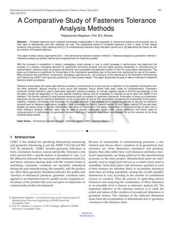
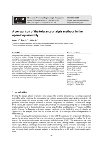
Kosec, Škec, Milerresult, the worst‐case tolerance chart method illustrates the minimal and maximal variation of afunctional requirement based on the values in the tolerance chain [9].When performing the tolerance chart method analysis, the first step is to set a goal by label‐ling the chain starting and ending points [16]. The starting point is selected on one edge and theending point on the opposite edge of the analysed feature (see Fig. 1). The chain indicator isplaced to determine the direction of the dimension vector and is either positive or negative [17].The vector pointing toward the chain end‐point is marked “ ”, and the vector pointing oppositeof the end‐point is marked “ “. The indicator shows whether to add or subtract dimensions andtolerances during the stack calculation. Additionally, it simplifies the interpretation of tolerancechart results [16]. The resulting dimension chain is the shortest possible and consists only ofknown dimensions ‐ dimensions set by designers.Tolerance chart method was used in recent studies [5, 6, 9, 15‐17], mostly as a reference forthe comparison of advanced tolerance analysis methods. Its most important advantage is sim‐plicity; no computational tools are needed as it can be carried out by hand. The downside is thatthe user has to keep in mind all the standard rules [2, 8] for creating the stacks, making the pro‐cess error‐prone. Besides, the tolerance chart method creates stacks in one direction and ignoresthe contributions of others, possibly providing unsatisfactory results.DescriptionDimension 1Dimension 2Dimension 3Dimension 4Sum TOL50501214935 1.5 0.5 0.7 0.2 2.95035 152.9Final dimension:15 2.9Fig. 1 Tolerance chart methodA plethora of statistical approaches was introduced to conduct non‐linear statistical toleranceanalysis. A typical example is the Monte Carlo simulation (MCS) based on the algorithm of thesame name. It utilises random sampling input values to calculate the output results. For a given, , ,. By using the math‐input vector , the number of sampling values is determinedematical model (transfer function)new output vector of same length is found, , ,. Finally, the output results are analysed by calculating statistical data such asmean, standard deviation, or range.Monte Carlo simulation (MCS) is a beneficial tool for tolerance analysis of mechanical assem‐blies. Its main advantage is flexibility and ability to use various non‐normal input or output dis‐tributions [18]. A large set of sample parts is created by randomly assigning a tolerance value toeach nominal dimension. Values are selected within the tolerance interval to simulate the manu‐facturing variation [18]. The process is repeated until enough output data is acquired to enablethe use of statistical techniques. It allows the calculation of the mean value, standard deviation,range, upper and lower specification limit, and share of rejected samples [19].Define the problemAnalyse the dataAssign the expectedtolerance distributionto each dimensionApply transfer functionEstimate the requirednumber of runsRandomly generatetolerances (at input)Fig. 2 Monte Carlo simulation for implicit assembly constraints46Advances in Production Engineering & Management 15(1) 2020
A comparison of the tolerance analysis methods in the open‐loop assemblyIn this article, MCS is applied as an extension to the Tolerance chart method. A modified formof MCS (McCATS) accounting for the implicit assembly variations was used, as suggested in [20].In the modified simulation, the random parts are sent to the assembly function, which iterativelysolves the tolerance chart equations for the dependent assembly variations [20]. The process isrepeated until a sample of a suitable size to produce the assembly histogram is created. Thesteps necessary to carry out the tolerance analysis using the MCS are shown in Fig. 2.The vector loop model is a stack‐up technique used to extend the stack analysis to two andthree‐dimensional assemblies [1]. The idea of the vector loop method is to use vectors to de‐scribe the dimensions and associated tolerances. Vectors are arranged in loops to determine theassembly deviations. Tolerance analysis problems are solved using the kinematic concept; con‐tact points are set as kinematic joints. A number of possible motions is defined for each joint (i.e.degrees of freedom), along with the local datum reference plane. Three types of variations aredescribed in vector loop model: dimensional variations (lengths and angles), kinematic varia‐tions (small adjustments between mating points, joints) and geometric/feature variations (posi‐tion, roundness, angularity) [1].Dimensional and geometric tolerances are described as additional degrees of freedom on thekinematic joints [1]. Kinematic simplification is required to represent geometric tolerances insuch way. Thus, in the vector loop model, geometric tolerances are included only at matingpoints, in the direction defined by the type of kinematic joint [1]. They are described as addi‐tional translational and rotational transformations (displacement vectors, rotation matrices) –as gaps with zero‐length nominal dimension vectors.The assembly graph is a diagram that represents the analysed assembly, including its parts,dimensions, mating conditions, functional elements, and functional requirements. The graph isused to represent any linear dimension in the assembly as a vector (see Fig. 3). Vectors are con‐nected and form chains or loops, reflecting how assembly parts stack‐up together. The associat‐ed tolerance is included as a small kinematic adjustment of such a vector (gap) [1, 12]. Such rep‐resentation allows us to determine the functional requirements of an assembly. Stack‐up func‐tions are built by including the vector variations involved in each chain into implicit kinematicequations. As such, they can then be solved using various mathematical approaches [1, 6].For each part in the tolerance chain, a local datum reference frame (DRF) is added to identifythe relevant features of a part for tolerance analysis. DRFs are then connected using datum pathsrepresenting geometric layouts, which define the direction and orientation of vectors formingthe loop [1]. They are created by stacking and chaining the dimensions that locate the contactpoint between two parts. After creating datum paths, the vector loops can be created by connect‐ing datums. Loops can be open or closed, depending on the functional requirement of the toler‐ance analysis. The number of closed loops is calculated as1, where is the numberof the mating points, and the number of parts.ggL3DSquareBoxL2CL1BCircleAFig. 3 Assembly graph and the example of vector loopsAdvances in Production Engineering & Management 15(1) 202047
Kosec, Škec, MilerAfter defining the vector loops, the calculation is carried out [1, 11]. When considering theclosed‐loop problem, the equations are often non‐linear; they must be linearized using directlinearization method [1, 11], producing approximate results. Thus, vector loop, when using di‐rect linearization, is unable to generate true worst‐case results [4, 11]. When the open‐loopproblem is considered, deviations are calculated directly using explicit equations [11].Unified Jacobian‐torsor (JT) method [21] is a 3D tolerance analysis method. It uses the Jaco‐bian matrix to relate the functional requirement (FR) and virtual joints displacements. JT ad‐vances the punctual small‐displacement variables of the Jacobian formulation to represent tol‐erance zones using the torsor model and interval arithmetic. It offers more output informationon the FR, reducing the size of the analysed model since it is no longer point‐based [21].Torsor model uses small displacement screws to establish tolerance zones of points, curves,and surfaces [21, 22]. Each real surface is modelled by a substitution surface defined by a set ofscrew parameters that are modelling the deviations from nominal geometry [23]. Screw param‐eters are arranged in torsors containing translational components of a point , ,and , ,as rotational components with respect to the nominal geometry:,(1)where is DRF used to evaluate the screw components. Torsor model can fully define the toler‐ance zones due to its ability to shape spatial volumes within which the surfaces are deviating [10].The procedure of Unified Jacobian‐torsor method consists of 4 steps [24]. The first step is toidentify all functional elements (FEs) affecting the FR by distinguishing kinematic chains involv‐ing the functional condition or part under study. Functional element can be any point, curve orsurface of a part and creates internal or kinematic pairs [21]. The second step is to associate atorsor or screw parameter to each element (surface, axis) of the kinematic chain. Torsors ex‐press the degrees of freedom and the allowable element displacements and their bounds. Smalldisplacements are applied to parts’ geometrical features affecting the FR [21], after which theJacobian matrix is used to determine relative positions and orientations of torsors within thechosen kinematic chain (step three) [22]. The final step is to combine torsor and Jacobian toprovide a matrix equation. Solving a resulting matrix using interval algebra provides the func‐tional condition bounds.2.2 Assembly model for case studyThe above‐described methods were compared by analysing a 3D tolerancing problem. The as‐sembly consisting of the cantilever and the rotating handle (open loop) was used as an example.Thus, both the dimensional and geometric tolerances were considered. The functional require‐ment deviations are assessed using each of the methods, while the results are compared in Sec‐tion 3.5. The nominal dimension (DIM), upper deviation limit (UDL), and lower deviation limit(LDL) were calculated. The comparison is focused on the similarities and differences betweenresults obtained by each method. Differences in procedures and calculation approaches are alsoobserved.A simple rotating handle assembly consisting of four parts was used to carry out the compari‐son between the methods (see Fig. 4). The pole (2) is fixed to the bottom plate (1), while thelever (3) is mounted onto the journal located on the pole. The handle (4) is installed into thebore located on the lever. Tolerances were assigned to all the dimensions apart from a distancebetween the handle (4) and the base plate (1), which is selected as a functional requirement).48Advances in Production Engineering & Management 15(1) 2020
A comparison of the tolerance analysis methods in the open‐loop assemblyFig. 4 Case study modelThe positional tolerance between the top surface of the base and its cut‐out was includ‐ed. The contact between the base and the cylindrical base of the pole is considered ideal. Theparallelism tolerance between the axis of the cylindrical pin located on the pole and the bottomsurface of the pole was also included. The lever is mounted onto the pole pin (see Fig. 4) byclearance fit 45 H8/g7. On the opposite side of the lever, the handle is mounted into the borewith a clearance fit 45 G6/h7. Regarding the geometric tolerances, the parallelism between twolever bores and perpendicularity between the handle and the mounting sleeve wall were re‐quired.Each method was then applied to the above‐described open‐loop assembly. The results werecompared according to three criteria: identification of the contributing tolerances,calculation of the dependent dimension (functional requirement),analysis of calculation differences compared to the assemblies with closed loops.An assembly graph was created for each of the methods except for the Monte Carlo simula‐tion, as it is based on Tolerance chart method.3. Results and discussion3.1 Tolerance chart resultsTolerance chart method is mostly used for dimensional tolerances, even though the recent modi‐fications have enabled the analysis of geometric tolerances as well [15]. The geometric toleranc‐es are to be transformed into their dimensional counterparts. Yet, such transformation does notaccount for the angular surface deviation. In this article, the tolerance chart method is appliedonly to dimensional tolerances.Tolerance chain consisting of base plate bore depth (a), length between the pole basis andpole journal axis (b), tolerance fit between pole journal and lever bore (c and d), distance be‐tween lever bore axes (e), and tolerance fit between lower lever bore and handle (f and g). Asmentioned, the distance between the top surface of the base plate (part 1) and handle (4) is afunctional requirement. Indices U and L were included to denote the upper and lower deviationlimit, respectively.Advances in Production Engineering & Management 15(1) 202049
Kosec, Škec, 5TOL.00cut –0.009/2; clt –0.034/2dut 0.039/2; dlt 00fut 0.025/2; dlt 0.006/2gut 0/2; glt ‐0.025/2210Nominal functional requirement dimension:152 mmStack equation for the upper deviation limit:0.008 mmStack equation for the lower deviation limit:0.062 mmFig. 5 Application of tolerance chart methodThe tolerance stack coordinate system is defined next; the starting point is set at the baseplate surface (1). The upward dimension is shown in Fig. 5 is selected as positive and markedwith the indicator “ ”, while the downward is negative and marked with “ ”. The direction ofthe tolerance chain is chosen arbitrarily, but it is important to respect the specified directionalong the chain. Finally, the results are calculated by adding and subtracting values along thetolerance chain and shown in Fig. 5.3.2 Monte Carlo simulation resultsMonte Carlo simulation was applied following the procedure explained in Section 2.1. Determin‐ing the appropriate distribution to each of the tolerances was the crucial step, as it affects theresults. The distribution of geometric tolerances along with the interval between the upper andlower deviation limit most frequently follows the normal distribution.Tolerance fits are asymmetrical, requiring the use of the skewed distribution according to[19]. Distribution of input values is described using 3 process range (6 ). Since data aboutthe manufacturing process was not available, 3DCS CATS software was used to determine thedistribution models of tolerance fits. According to 3DCS, tolerance fits have unimodal continuousprobability distribution called Pearson 1. Since tolerance limits assigned to dimension c are neg‐ative, the distribution model is skewed left from the nominal dimension. The same can be con‐cluded for the tolerance assigned to dimension g. On the other hand, tolerance limits assigned todimensions d and f are positive, and distribution is right‐skewed.RunsNominalMeanSTD6STDLSLUSLEST. TYPEEST. LOWEST. HIGHEST. RANGE2000152.000 mm151.999 mm0.018 mm0.110 mm151.000 mm153.000 mmPearson I151.958 mm151.995 mm0.085 mmFig. 6 Monte Carlo assembly results and histogram50Advances in Production Engineering & Management 15(1) 2020
A comparison of the tolerance analysis methods in the open‐loop assemblyNext step is to define the variation model function. Since Monte Carlo is applied to tolerancechart method, tolerance stack equations are used to define it. After running the simulation for 2000 times with randomized input variables, an output model for FR was created. A variationanalysis provides descriptive statistics, inferential statistics data, and a histogram (shown in Fig.6). By adding and subtracting the input variables using the variation model functions, distribu‐tion of FR tolerances was found. The resulting functional requirement distribution is also Pear‐son 1. However, it is not as profoundly left‐ or right‐skewed as are the input variables.3.3 Vector‐loop resultsAn assembly graph describing the open‐loop of the assembly and its vector loop tolerance chain(or datum path) was created. It was used to identify of the number of vector chains and loopsinvolved in the assembly (Fig. 4). Since each part is in contact with its two neighbouring partsonly once, this assembly contains one open loop. Same can be seen on the assembly graph (Fig. 7)where each arrow is representing the contact between parts. Vector loop is open at the gap(noted g) between the Handle (Part 4) and Base (Part 1).The datum path (Fig. 7, right) connects the point, surface, axis or DRF of a part with nextpart’s point, surface axis or DRF. DRFs have been assigned to each part with respect to the origincoordinate system at the top of the Base (Part 1). All the DRFs have a horizontal ‐axis and verti‐axis corre‐cal ‐axis. Origin coordinate system is set in such a way that positive direction ofsponds with the positive direction of a tolerance chain in Tolerance chart method. This eases thetracking and method comparison.The geometric tolerances were also accounted for. Each tolerance was represented as an ad‐ditional vector of magnitude equal to /2, where is the width of corresponding tolerance field(see Fig. 4; 0.2 for the positional, and 0.1 for parallelism and perpendicularity tolerances). Theadditional vectors represent gaps between parts contacting points and were denoted based onthe corresponding nominal dimension. The position tolerance on the Base cut‐out with respectto the datum A (apos) is represented as a translation vector of the surface in the ‐direction (Fig.), and Lever holes () with respect to the7). The parallelisms applied to the Pole’s pin (datum B were also represented as translation vector along the ‐axis [1]. Perpendicularity ap‐) with respect to the datum D can be described asplied to the horizontal axis of the Handle (a translation along ‐axis [1]. According to the assembly graph there are3 contacting pointsand4 parts, resulting in 0 closed loops (Eq. 1 was used). There is also one open‐loop func‐tional requirement.Var.aposbparcdddeparfdgdhparTol. descriptionPosition (Base top to cutout)Parallelism (Pole’s to bottom)Dimensional tol. (Pole’s pin)Dimensional tol. (Lever’s upper hole)Parallelism (Lever hole axes)Dimensional tol. (Lever’s lower hole)Dimensional tol. (Handle)Perpendicularity (Handle axis)Gap vector length 0.1 0.05cdu –0.009; cdl –0.034ddu 0.039; ddl 0 0.05fdu 0.025; fdl 0.009fdu 0.0; fdl –0.025 0.05Uppervalue of functional requirement:22152.241 mm22Lower value of functional requirement:2222151.680 mmFig. 7 Vector loop assembly graph and resultsAdvances in Production Engineering & Management 15(1) 202051
Kosec, Škec, Miler3.4 Unified Jacobian‐torsor resultsBefore creating the assembly graph (Fig. 8), it was necessary to identify the functional elements(FE) and functional requirements (FR). Also, it was required to differentiate between the inter‐nal and kinematic pairs. For the assembly at hand, there are four internal and one kinematicpair. First internal pair (FE0‐1) is located on the Base (Part 1), as the positional tolerance definedbetween its top and cut‐out surface corresponds to functional surfaces 0 and 1 on the assembly.The parallelism tolerances define FE2‐3 and FE4‐5. Internal pair FE6‐7 is defined by the perpendicu‐larity tolerance set on the Handle (Part 4).Only kinematic pair (FE1‐2) is set between the Base cut‐out and Pole’s bottom. However, thecontact is assumed to be ideal so that it will not impact the analysis. Two more contacts definedby tolerance fits (between Pole and Lever, and between Lever and Handle) were not set as kin‐ematic pairs even though they are in physical contact. This means they are defined as importantconditions to be satisfied between two FEs. So, according to [13], they are then defined as func‐tional requirements that will be taken into account in the analysis as kinematic pairs.Upper value of functional requirement:152.28 mmLower value of functional requirement:151.143 mmFig. 8 Jacobian‐torsor method and resultsJacobian matrix and small‐displacement torsor vector were calculated for each internal andkinematic pair. A small‐displacement torsor vector was also calculated for each FE (based ontorsor representing the tolerance zone [21]):,(2)For each tolerance, translational and rotational components inside the tolerance zone weredetermined [21]. Since the direction of a functional requirement is along the ‐axis and rotationsthat would influence functional requirement are around and ‐axis, , and componentmust be calculated.Contact between functional surfaces 0 and 1 in the FE0‐1 is a planar contact with normal con‐taining one translation component ( ) and two rotational components ( , ) [12, 21]. Compo‐nents are calculated using the equations for planar surface according to [21]. Internal pairs FE2‐3,FE4‐5, and FE6‐7, and functional requirements FR3‐4 and FR5‐6 are defined by the tolerance fits.They use translational components v and w and rotational components and of a slipping piv‐ot with the axis [21]. Below is a table containing displacements torsors for each internal andkinematic pair.52Advances in Production Engineering & Management 15(1) 2020
A comparison of the tolerance analysis methods in the open‐loop assemblyTable 1 Displacement torsors for each internal and kinematic 40.0003 003 0.00040.0040.0040.0020.00040.0010.00100000Jacobian matrix is calculated according to the procedure presented in [21]. Its purpose is tocalculate the effect of the traditional torsor set for each functional element (FE) on the functionalrequirement (FR) of the assembly [21]. Finally, after calculating small‐displacement torsor vec‐tors and Jacobian matrices for each FE, the same can be done for FR: 0.058 0.2390.434 0.184.0.0010.0010.0050.0110.0040.010(3)3.5 Comparison of the results obtained by different methodsAfter analysing the assembly presented in Section 3.1 using the four methods, results are pre‐sented in Table 2. Abbreviations are used to ease the result disambiguation; TC was used fortolerance chain method, MC for Monte Carlo simulation, VL for the vector loop method, and JTfor the Unified Jacobian‐torsor method. Since it is not possible to include geometric tolerances inTC and MC
steps necessary to carry out the tolerance analysis using the MCS are shown in Fig. 2. The vector loop model is a stack‐up technique used to extend the stack analysis to two and three‐dimensional assemblies [1]. The idea of the vector loop method is to use vector