Transcription
SUPPLEMENTARY METHODSAnimal modelsFUCCI mice (B6;129-Gt(ROSA)26Sor<tm1(Fucci2aR)Jkn> stock No. RBRC06511)1on C57Bl/6 background were purchased from Riken (Japan) and maintained with ahomozygous/homozygous breeding scheme. To generate mice expressing the FUCCIreporters (mCherry and mVenus) only in podocytes, we used a mouse expressing theCre recombinase under the podocyte-specific NPHS2 promotor (129S6.Cg-Tg(NPHS2cre)295Lbh/BroJ, stock No. 008523; from Jackson Laboratory). The WT-POD-FUCCImice were generated by crossing 129S6-podocin-cre and the Fucci2aR mice (Fig 1a).We bred the WT-POD-FUCCI with our well characterized model of CKD, Alportsyndrome2-4 (B6.Cg-col4α5tm1Yseg/J , stock No. 006183; Jackson Laboratory), to studyspecifically cell cycle in podocytes in progressive CKD, and generated the AS-PODFUCCI mice. Alport colonies were maintained with a homozygous/hemizygous breedingscheme.Blood collection, creatinine, proteinuria measurementFrom facial vein puncture, blood samples (30µL) from all experimental mice werecollected using plasma separation tubes with lithium heparin (BD microtainer ,#365987). Serum creatinine was measured by colorimetric assay (BioAssay Systems,#DICT-500). Urine samples were collected as a spot sample. The urine albumin-tocreatinine ratio was determined using an ELISA assay for mouse albumin (ImmunologyConsultants Laboratory, #E90AL) and a quantitative colorimetric assay kit for urinecreatinine (BioAssay Systems, #DICT-500), performed following manufacturer's protocol.Tissue preparationAfter CO2 inhalation, intracardiac perfusion with PBSx1 (20mL) followed by CollagenaseI/IV/dispase mix was performed. Both kidneys were harvested, and the capsulesremoved. Cortical tissue was minced for 5 minutes and then digested at 37 C incollagenase mix (collagenase type I 200U/mL, Worthington, #LS004196, and type IV200U/mL, Worthington, #LS004188, and dispase 0.95U/mL, Worthington, #LS02104) in
RPMI medium (#A1049101). The lysate was passed through 100 µm and 30 µm nylonmesh filters. Blood lysate kit (Miltenyl Biotech, #130-094-183) was used to removeerythrocytes. For each sample, the single cell suspension was resuspended in 85µL of5% bovine serum albumin (BSA) for 30 minutes for blocking. Antibody against nephrin(1.5µg /107 cells, Abcam, #136894) was conjugated with 7.5µL of Zenon AlexaFluor 647Rabbit IgG Labeling kit (Invitrogen, #Z25308) before adding it to the single cellsuspension for 1h at 4 C. Samples were washed with PBSx1 and resuspended in 400µLof PBSx1 for analysis and sorting.Flow cytometry and gating strategyCells were sorted using a 70 µm nozzle and an event rate of 1000/s. 647 nmfluorochrome, mCherry and mVenus positive cells were quantified using a cytoflex flowcytometer with far red (640 nm); yellow (561 nm) and blue (488 nm) lasers respectivelywith 660/20 (647 fluorochrome), 575/26 (mCherry) and 530/30 (mVenus) filters. Cellswere collected in sorting buffer and then washed and resuspended in RIPA (protease andphosphatase inhibitor) buffer for further analysis. The gating strategy is described inSuppl. Fig.1. We first gated for the population positive for 647 fluorochrome (nephrin) andunder this population we analyzed the expression of FUCCI fluorochrome signals(mCherry and mVenus). One and one-half kidney was used for FACS (the remaining halfa kidney was used for histology studies). 200000 events were run to determine cell cycledistribution.Immunofluorescent stainingFrom the same mice used for FACS, a quarter of kidney tissue was fixed, dehydrated inalcohol, and paraffin embedded. For immunohistochemistry, after samples wererehydrated and deparaffinized, heat-mediated antigen retrieval was performed in acitrate-based solution (Vector laboratories, #-3300-250) on thin deparaffinized kidneysections (4 µm). The sections were blocked in PBS 1X containing 2% serum bovinealbumin (Jackson ImmunoResearch Lab, #001-000-162) for 15 minutes at roomtemperature and incubated with antibody against mCherry fluorochrome (Thermofisher,#M11217) at 1:100 dilution, mVenus (myBiosource, #MBS448126) at 1.5:100 dilution,
nephrin (SantaCruz, #SC-377246) at 1:50 dilution followed by secondary antibody at1:500 dilution. Sections were counter mounted with DAPI (Vector Laboratories, #H-120010). A Leica DM fluorescent microscope was used in conjugation with Open Lab 3.1.5software for image capture. The same protocol was followed for staining human paraffinsection of the human AS patient with PDlim2 (ThermoFisher, # PA5-52009; at 1:100dilution).Western Blot analysisUpon sorting, podocytes were immediately washed and resuspended in RIPA buffer forsubsequent proteomic and western blot analysis. Protein samples (20 µL) were loadedinto pre-made gel for migration under 100V and then transferred onto a polyvinylidenefluoride 0.45 µm membrane (Trans-Blot Turbo Midi 0.2 µm PVDF Transfer Packs,BioRad, #1704157). Blotted membranes were blocked with 5% dry fat milk containing50mM Tris-HCl buffer (pH 7.5) and 150 mM NaCl for over 1h then blotted overnight incold room with WT-1 antibody (Abcam, # 89901), b-actin (GTX, #109639). b-actin wasused as the housekeeping protein.Primary podocyte extractionPrimary podocytes were also selected with an alternative method (magnetic beadsselection) to sort for in vitro experiments. We used the same nephrin antibody (Abcam,#136894,) and we confirmed the expression of nephrin in podocytes selected to validateisolation method of the same population. Kidneys were processed and digested to singlecell solution as described previously. After adding 100 µL of BSA for 30 min on ice, 3 µLrabbit nephrin antibody (same as previous) was adding to each sample for 45 minutes.Cells were then mixed with anti-rabbit IgG microbeads for 20 minutes at 4 C (MiltenyiBiotec, #130-048-602). Magnetic separation was done using MACS Column (MiltenyiBiotec, #130-042-201) for positive selection5. The targeted cells were collected accordingto the product protocol. 3,000 primary podocytes were then plated for 4 days in VRADmedium6-7 before starting in vitro experiments.Podocytes were then fixed with paraformaldehyde 4% and serial washes with PBS andthen permeabilized with Saponin 0.1%, blocked with 5% bovine serum albumin and thenreacted with nephrin antibody overnight. Cells were washed and slides were mounted
with DAPI (Vector Laboratories, #H-1200-10). Confocal z-stacks images were acquiredwith an LSM 700 system mounted on an AxioObserver.Z1 microscope. GFP andmCherry fluorescence was excited with 488 nm and 555 nm laser light. Images wereprocessed using the ZEN10 software (blue edition; Carl Zeiss Microscopy).Puromycin aminonucleoside in vitro experimentAfter 4 days in culture in VRAD medium, medium was replaced with VRAD modifiedmedium (without dexamethasone). Three conditions were applied, either PAN (5, 15, or35 µg/mL, Sigma Aldrich, #58606, SBR 00017, 10mg/mL) or control VRAD modifiedmedium for 72hours. Imaging was acquired during the experiment and after 72hours ofculture, cells were analyzed through FACS as described earlier.Glomeruli imagingConfocal images of fixed glomeruli were acquired on LSM 700 and LSM 710 systemsmounted on AxioObserver.Z1 microscopes equipped with Plan-APOCHORMAT 20x/0.8lenses (Carl Zeiss Microscopy).GFP and mCherry fluorescence was sequentially excited with 488 nm and 555 nmlaser light, respectively. Brightfield images were acquired with a transmitted lightdetector simultaneously with the mCherry fluorescence channel using the same 555 nmlaser light. The pinhole was set to 1 Airy unit (34 um for GFP and mCherry and 29 umfor DAPI) and z-stack spacing was 3 um.Podocyte number evaluationCortical tissue from mice was harvested at 2, 4 and 6 months and was fixed and preparedas above. In addition to staining for WT1 [(Abcam, #ab15249), the glomerular basementmembrane was stained using wheat germ agglutinin (WGA, Vector, #RL-1022) with anAlexa-Fluor conjugate. Sections of cortex were imaged at 40x with OpenLab 3.1.5. Thenumber of podocyte (WT1 ) nuclei per glomerular cross-section was counted and theglomerular tuft area (WGA ) was measured by planimetry using ImageJ. With constantsection thickness, the areal density (NA) of podocytes per tuft area is directly proportionalto the volumetric density (NV), podocytes per tuft volume8-9. Glomerular tuft volume VG
was estimated using the Weibel formula10 from the mean glomerular tuft area (AG): VG (b/d) AG3/2, where b is a shape coefficient (1.382 for spheres) and d is the sizedistribution coefficient accounting for variation in tuft size (typically 1.1 is used). The indexNA VG is directly proportional to the number of podocytes per glomerulus. The permouse average NA was calculated from the individual glomerular values weighted by thetuft area.Proteomics sample preparation and LC-MS/MS analysisCell populations were obtained in biological replicates for WT G0, AS G0, and AS G1. 10,000 cells were used to perform the nanoProteomics profiling of the cells using aprotocol adapted from the μPOTS protocol previously described11. Briefly, a lysis bufferwas created using 0.05% n-dodecyl β-D-maltoside (DDM, Thermo Scientific). Afteradding 10 µL of chilled lysis buffer, the samples were incubated in a thermomixer set for30 minutes at 25 C and 300 rpm. Once complete the samples were reduced with 5 mMdithiothreitol (DTT) (Sigma-Aldrich) for 30 minutes at 37 C and 300 rpm. Reducedcystines were alkylated with 10 mM iodacetamide (IAA) (Sigma-Aldrich) for 30 minutes at25 C and 300 rpm in the dark. These samples were double digested first using 10 ngtrypsin (Promega) that was diluted with 100 mM HEPES and were incubated for 2hoursat 25 C and 300 rpm. After the initial digest the samples received 25 ng of trypsin(Promega), followed by a 14-hour incubation set at 25 C and 300 rpm. All the sampleswere then quenched and diluted to a final volume of 35 µl and transferred to apolypropylene vial.A homebuilt LC system was employed to automatically perform sample injection, samplecleanup, and LC separation12. Both SPE trapping (150 µm i.d., 4-cm length) and LCcolumn (50 µm i.d., 60-cm) were slurry-packed with Jupiter C18 packing material (300-Åpore size, trapping column 5 µm, and analytical column 3-µm particle sizes). The samplewas injected into a 20-µL loop and loaded onto the trapping column using Buffer A (0.1%formic acid in water) at 3 µL/min for 20 min. After trapping, the sample was reverse-floweluted onto the analytical column at 150 nL/min and separated by a gradient of 5–8% (0–2 min), 8–12% (2–20 min), 12–35% (20–75 min), and 35–60% (75–97 min) of Buffer B(0.1% formic acid in acetonitrile). The LC column was then washed using 75% Buffer B
for 10 min and re-equilibrated using 5% Buffer B for 50 min. All data were acquired usingan Orbitrap mass spectrometer (ThermoFisher) under automated data dependentacquisition mode. The mass spectrometry proteomic data have been deposited to theProteomeXchange Consortium via the MassIVE partner repository with the datasetidentifier MSV000086705.The spectral identifications were performed using MaxQuant (v1.6.0.16) using the defaultparameters except the following: trypsin was set as digestion enzyme, Label freequantification and iBAQ were active and match between run was enabled with a matchingtime window of 1.5 min. Methionine oxidation and N-terminal acetylation were set asvariable modification and cysteine carbamidomethylation was set as fixed modifications.The data was searched against Mus musculus UniProt redundant database(UP000000589 downloaded in May 2020, 55,421 sequences). The subsequent dataprocessing of the protein iBAQ intensities was performed in R v4.0.2 using the packageRomicsProcessor v1.0.0, which is available on GitHub ssor)13 and Protein-Mini-On, a package developed to performedenrichment analysis for GO terms and KEGG pathways. The code to perform the analysiswas also uploaded on GitHub to make the data analysis reproducible(https://github.com/GeremyClair/Effect of glomerular disease on the podocyte cell cycle) and as Supplementary DataSet 07. The results of the analysis are provided in anexcel document (Supplementary Dataset 01-06). Briefly the data was log2 transformed,median centered. Only the proteins detected in 2/3 samples of a given condition wereconsidered for quantification. PCA and hierarchical clustering were performed to verifythe grouping of the sample within each condition. Missing values were imputed usingrandom values drawn from a normal downshifted from the data distribution. ANOVA andStudent’s t-tests were performed. The p-value frequency was plotted to ensure that thep 0.05 threshold was selected appropriately. Enrichment analysis were performed usingFisher’s Exact test by comparing the lists of protein of interest to the proteins that weredetectable by the methods employed.
REFERENCES1. Mort RL, Ford MJ, Sakaue-Sawano A, et al. Fucci2a: A bicistronic cell cyclereporter that allows Cre mediated tissue specific expression in mice. Cell Cycle.2014;13(17):2681-2696.2. Sedrakyan S, Da Sacco S, Milanesi A, et al. Injection of Amniotic Fluid Stem CellsDelays Progression of Renal Fibrosis. J Am Soc Nephrol. 2012;23(4):661-673.3. Soloyan H, Thornton M, Villani V, Khatchadourian P, Cravedi P, Angeletti A,Grubbs B, De Filippo RE, Perin L, Sedrakyan S. Glomerular endothelial cellheterogeneity in Alport syndrome. Sci. Rep. 2020; 10: 11414.4. Rheault MN. Mouse Model of X-Linked Alport Syndrome. J Am Soc Nephrol.2004;15(6):1466-1474.5. Murakami A, Oshiro H, Kanzaki S, et al. A novel method for isolating podocytesusing magnetic activated cell sorting. Nephrol Dial Transplant. 2010;25(12):38843890.6. Takano Y, Yamauchi K, Hiramatsu N, et al. Recovery and maintenance of nephrinexpression in cultured podocytes and identification of HGF as a repressor ofnephrin. Am J Physiol-Ren Physiol. 2007;292(5):F1573-F1582.7. Da Sacco S, Lemley KV, Sedrakyan S, et al. A novel source of cultured podocytes.PloS One. 2013;8(12):e81812.8. Lemley KV. Simplification of the Weibel- Gomez method for estimating podocytenumber. Stereology and Image Analysis. Proceedings of the ECS10, V Capassoet al. Bologna, Italy. Published online 2009.9. Lemley KV, Bertram JF, Nicholas SB, White K. Estimation of Glomerular PodocyteNumber: A Selection of Valid Methods. J Am Soc Nephrol. 2013;24(8):1193-1202.10. Weibel ER: Stereological Methods. 1. Practical methods for biologicalmorphometry. pp 44-45. New York, Academic Press, 1979.11. Xu K, Liang Y, Piehowski PD, et al. Benchtop-compatible sample processingworkflow for proteome profiling of 100 mammalian cells. Anal Bioanal Chem.2019;411(19):4587-4596.
12. Zhao R, Ding SJ, Shen Y, et al. Smith Automated metal-free multiple-columnnanoLC for improved phosphopeptide analysis sensitivity and throughput. JChromatogr B Analyt Technol Biomed Life Sci. 2009; 877(8-9): 663–670.13. Dou M, Clair G, Tsai C-F, et al. High-Throughput Single Cell Proteomics Enabledby Multiplex Isobaric Labeling in a Nanodroplet Sample Preparation Platform. AnalChem. 2019;91(20):13119-13127.
Supplementary Figure 1Supplementary Figure 1. Gate Strategya. Cells were first gated based on forward scatter (FSC-A) and side scatter (SSC-A) areasto exclude dead cells and potential cellular debris from the analysis (P1). b-c. Furthergating was performed to remove duplets based on FSC-H/FSC-W (P2) and SSC-H/SSCW (P3). d-e. Histogram plot (gated on APC/Alexa-Fluor-647, d) and quadrant plot (gatedon PE/mCherry and FITC/mVenus, e) were established on P3 gate based on theunstained events for each channel. f. The same strategy used in a-e was applied toanalyze the cortical cells. First, cells were selected by nephrin expression (AF-647, P4,g) from this population, P4, the expression of mCherry(Q4) /mVenus signal (Q1) wasanalyzed (h). Gating was performed following the same criteria but independently foreach sample to reflect differences between the analyzed population.
Supplementary Figure 2Supplementary Figure 2. Podocytes enters cell cycle G1 phase during CKDprogressiona-d. Representative immunofluorescence image showing expression of FUCCIfluorescences markers, mCherry (red), mVenus (green), Dapi in glomerulus extractedfrom (a) WT-POD-FUCCI mice, (b) AS-POD-FUCCI male mice at 2 months, (c) AS-PODFUCCI male mice at 4 months and (d) AS-POD-FUCCI male mice at 6 months. Scalebar: 50 µm. The number of podocytes in G1 phase (*) increase over time. e-h.Representative immunofluorescence image showing decrease of podocytes number,identified by WT1 (fushia) expression, with nuclear staining Dapi (blue) and glomerularbasal membrane staining using WGA staining (green) in AS male mice at 2, 4 and 6months compare to WT mice (4 months, male). Scale bar: 100 µm.
Supplementary Figure 3Supplementary Figure 3. Gate strategy applied to select G0 podocytes and G1podocytes in WT and AS micea. Cells were first gated on forward scatter (FSC-A) and side scatter (SSC-A) areas toexclude dead cells and potential cellular debris (P1). b-c. Further gating performed toremove duplets based on FSC-H/FSC-W (P2) and SSC-H/SSC-W (P3). d. quadrant plot(gated on PE/mCherry and FITC/Venus) were established on P3 gate based on unstainedevents for each channel. e. Histogram plot (gated on APC-Alexa-Fluor-647-nephrin). f.The same strategy used in a-e was applied to analyze the cortical cells from WT PODFUCCI mouse at 6 months. g. To select WT podocytes (pod) in G0, cells were firstselected cells by negative expression of FUCCI signal (Q3-2). From this population, cellsexpressing nephrin (APC-AF647-A) were sort in group WT G0. WT-G1 population wasselected as cells expressing mCherry. h. The same gate strategy was applied forselecting cells from AS-POD-FUCCI male mice at 6months. Cells negative for FUCCImarkers (Q3-2) were selected (i). From this population (Q3-2) cells expressing nephrinP6-G0 for the group AS G0 podocytes were selected. Cells expressing mCherry wereselected to collect AS G1 podocytes.
Supplementary Figure 4Supplementary Figure 4. Unsupervised Principal Component Analysis in WT G0,AS G0 and AS G1a-f. Unsupervised Principal Component Analysis (PC1 in a, PC2 in c, and PC3 in d) basedon label-free quantitation of the proteins expressed in WT G0, AS G0 and AS G1.Percentage of total variance is indicated after each principal component. In b isrepresented a list of significantly enriched GO terms (Fisher’s exact p 0.05) for the list of10% proteins significantly higher or lower in abundance in PC1. In e is represented a listof significantly enriched GO terms (Fisher’s exact p 0.05) for the list of 10% proteinssignificantly higher or lower in abundance in PC2. In f is represented a list of significantly
enriched GO terms (Fisher’s exact p 0.05) for the list of 10% proteins significantly higheror lower in abundance in PC3. Because of space limitations the complete results couldnot be depicted on this figure and is provided as Supplementary Dataset 03.Supplementary Figure 5Supplementary Figure 5. Volcano plot representing the results of comparison ofthe proteome of AS G1 and WT G0 podocytesThe proteins significantly higher in abundance in AS G1 vs. WT G0 are represented inblue; the proteins significantly lower in abundance in AS G1 vs. WT G0 are representedin yellow; the blue and orange boxes contain a list of significantly enriched GO terms andKEGG pathways (Fisher’s exact p 0.05) for the lists of proteins significantly higher orlower in abundance in G1 respectively. Because of space limitations the complete resultscould not be depicted on this figure and is provided as Supplementary Dataset 5.
Supplementary Figure 6Supplementary Figure 6. Selection of GO terms and KEGG pathways enriched forthe group of proteins modulated solely in one of the three group comparisonsThe Venn diagram is the same as depicted in Fig 4 e. The content of the teal, gold, andpink boxes is a selection of GO terms and KEGG pathways enriched (Fisher’s exactp 0.05) in the list of proteins solely modulated in one of the three following comparisons:AS G1 vs. AS G0 (teal), AS G1 vs. WT G0 (gold), and AS G0 vs. AS G0 (pink).Because of space limitations the complete results could not be depicted on this figure andis provided as Supplementary Dataset 06.
Supplementary DataSet 07Cell cycle alport proteomicsRequired librariesThe required libraries are loaded - RomicsProcessor written by Geremy Clair (2020) is used toperform trackable transformation and statistics to the dataset - proteinminion written byGeremy Clair (2020) is used to extract fasta information and to perform gene ontology andKEGG pathways enrichement analysis (in prep ion")library("DT") #for the rendering of the enrichment tableslibrary("eulerr") #for the venn and euler diagramsFasta and protein ontologies download using ‘Protein Mini-On’Using the package ‘Protein Mini-on’ (Geremy Clair 2020, in prep.), The fasta file wasdownloaded from Uniprot.if(!file.exists("./03 Output files/Mus musculus proteome up000000589 2020 0713.fasta")){download UniProtFasta(proteomeID "up000000589", reviewed F, export T, file "./03 Output files/Mus musculus proteome up000000589 2020 07 13.fasta")}Then we’ve extracted and parsed the details contained in the fasta file header into a tablecontaining a list of details for each protein.if(!file.exists("./03 Output files/UniProt Fasta info.csv")){write.csv(UniprotFastaParser(file "./03 Output files/Mus musculus proteomeup000000589 2020 07 13.fasta"),file "./03 Output files/UniProt Fasta info.csv")}For each entry, ‘Protein Mini-On’ was use to download Gene Ontology (GO) terms and KEGG idsassociated with the proteins. This upload was performed the exact same day as the downloadof the fasta file was done to ensure that the IDs will be identical as the ones present in the fastafile used).if(file.exists("./03 Output files/UniprotTable Mus musculus proteome up000000589 2020 07 13.csv")){UniProtTable -read.csv("./03 Output files/UniprotTable Mus musculus proteome up000000589 2020 07 13.csv")
}else{download UniProtTable(proteomeID "up000000589", reviewed F)write.csv(UniProtTable,("./03 Output files/UniprotTable Mus musculus proteome up000000589 2020 07 13.csv"),row.names FALSE)}‘Protein-Mini-on’ was then used to generate a table (UniProtTable) containing the list of GOsand their associated protein IDsif(file.exists("./03 Output files/UniProtTable GO.csv")){UniProtTable GO -read.csv(file "./03 Output files/UniProtTable GO.csv")}else{generate UniProtTable GO()write.csv(UniProtTable GO,file "./03 Output files/UniProtTable GO.csv",row.names FALSE)}‘Protein-Mini-on’ was used to download similar information from KEGG for the Pathwaysassociated with each proteinif(file.exists("./03 Output files/UniProtTable KEGG.csv")){UniProtTable KEGG -read.csv(file "./03 Output files/UniProtTable KEGG.csv")}else{generate UniProtTable KEGG()write.csv(UniProtTable KEGG,file "./03 Output files/UniProtTable KEGG.csv",row.names FALSE)}MaxQuant importThe data was searched in MaxQuant using the mouse database generated above using the LFQquantification and Match Beetwen Runs (MBR) algorithm, the parameter.txt file indicates theparameters employed.data -extractMaxQuant("./01 Source files/proteinGroups.txt",quantification type "iBAQ",cont.rm T,site.rm T,rev.rm T)## [1] "70 Proteins were removed (protein(s) only identified by site,contaminant(s),reverse hit(s))"## [1] "iBAQ quantification was used"write.csv(data,file "./03 Output files/data raw.csv")IDsdetails -extractMaxQuantIDs("./01 Source files/proteinGroups.txt",cont.rm T,site.rm T,rev.rm T)## [1] "70 Proteins were removed (protein(s) only identified by site,contaminant(s),reverse hit(s))"IDsdetails -cbind(UniProt Name sub(".*\\ ","",IDsdetails protein.ids), IDsdetails)
write.csv(IDsdetails,file "./03 Output files/IDs details.csv")colnames(data) - sub("iBAQ.","",colnames(data))data[,1] - sub(".*\\ ","",data[,1])metadata - read.csv(file "./01 Source files/metadata.csv")colnames(metadata) -tolower(colnames(metadata))Romics object creationThe data and metadata were placed in an romics object, the sample names were retrievedfrom the metadata, the condition will be use for the coloring of the Figures.romics proteins - romicsCreateObject(data, metadata,main factor "Condition")Data cleaning and normalizationThe zeros were replaced by missing valuesromics proteins -romicsZeroToMissing(romics proteins)The proteins to be conserved for quantification were selected to contain at least 60% ofcomplete value for a given condition (2/3 sample of a given condition at least), the overallmissingness was evaluated after filtering.romics proteins -romicsFilterMissing(romics proteins,percentage completeness 60)## [1] "238 rows were removed for the data"## [1] "Based on the minimum completeness set at 60%"## [1] "at least the following number of sample(s) containing data was required:"## A G0 A G1 WT G0##222print(paste0(nrow(romics proteins data),"/", nrow(romics proteins original data)," proteins remained after filtering", " (",round(nrow(romics proteins data)/nrow(romics proteins original data)*100,2),"%)."))## [1] "2151/2389 proteins remained after filtering (90.04%)."The data was log2 transformed, the distriution boxplot were then plottedromics proteins -log2transform(romics proteins)distribBoxplot(romics proteins)
As the same quantity of protein was labelled for each sample, the expectation is that thedistribution of the protein abundance is centered, therefore a median centering was performedprior to plot again the distribution boxplots.romics proteins -medianCenterSample(romics proteins)distribBoxplot(romics proteins)
Data imputationFor some of the subsequent statistics imputations are required, we performed an imputationby assuming that the “non-detected” proteins were either low abundance or missing using themethod developped by Tyranova et al. (PMID: 27348712). The gray distribution is the datadistribution, the yellow distribution is the one for the random values used for imputation.imputeMissingEval(romics proteins,nb stdev 2,width stdev 0.5, bin 1)romics proteins -imputeMissing(romics proteins,nb stdev 2,width stdev 0.5)The PCA grouping were checked after imputationindPCAplot(romics proteins, plotType "percentage")
indPCAplot(romics proteins, plotType "individual",Xcomp 1,Ycomp 2,label F)indPCAplot(romics proteins,F)plotType "individual",Xcomp 1,Ycomp 3,label
indPCA3D(romics proteins)We will extract the contributions of the proteins to the 3 first componentsPCA results -romicsPCA(romics proteins)PCA var coord -data.frame(PCA results var coord[,1:3])colnames(PCA var coord) -c("PC1","PC2","PC3")ggplot(PCA var coord, aes(x PCA var coord[,1], y PCA var coord[,2])) geom point(size 3,alpha I(0.5)) xlab("PC1") ylab("PC2") ggtitle("Principal component analysis protein contributions") theme ROP()
ggplot(PCA var coord, aes(x PCA var coord[,2], y PCA var coord[,3])) geom point(size 3,alpha I(0.5)) xlab("PC2") ylab("PC3") ggtitle("Principal component analysis protein contributions") theme ROP()We’ve extracted the top10% proteins contributing the most to each PCA axis
tenpercentproteins -round(nrow(PCA var coord)*10/100,digits 0)print("Proteins contributions to PC1")## [1] "Proteins contributions to PC1"top10percentPC1 -PCA var coord[1]top10percentPC1 names -rownames(top10percentPC1)top10percentPC1 C1) -gsub(";.*","",top10percentPC1 names)top10percentPC1 -abs(top10percentPC1)top10percentPC1 -top10percentPC1[order(top10percentPC1,decreasing T)]datatable(data.frame(abs contrib top10percentPC1))top10percentPC1 ("Proteins contributions to PC2")## [1] "Proteins contributions to PC2"top10percentPC2 -PCA var coord[2]top10percentPC2 names -rownames(top10percentPC2)top10percentPC2 C2) -gsub(";.*","",top10percentPC2 names)top10percentPC2 -abs(top10percentPC2)top10percentPC2 -top10percentPC2[order(top10percentPC2,decreasing T)]datatable(data.frame(abs contrib top10percentPC2))top10percentPC2 ("Proteins contributions to PC3")## [1] "Proteins contributions to PC3"top10percentPC3 -PCA var coord[3]top10percentPC3 names -rownames(top10percentPC3)top10percentPC3 C3) -gsub(";.*","",top10percentPC3 names)top10percentPC3 -abs(top10percentPC3)top10percentPC3 -top10percentPC3[order(top10percentPC3,decreasing T)]datatable(data.frame(abs contrib top10percentPC3))top10percentPC3 rse -gsub(";.*","",rownames(PCA var coord))write.csv(top10percentPC1,"./03 Output C2,"./03 Output C3,"./03 Output files/top10percentPC3.csv")Now let’s perform enrichment analysis to evaluate the function participating the most to theseseparations
PC1 top10 enrich - cbind(Type "GO top10% PC1", UniProt GO Fisher(top10percentPC1,universe))## [1] "Your query contained 0 UniProt IDs and 215 UniProt Accession (somemight be redundant)."## [1] "The uniprot Accession of your query were converted in Uniprot IDs."## [1] "Your universe contained 0 UniProt IDs and 2150 UniProt Accession (some might be redundant)."## [1] "The uniprot Accession of your universe were converted in Uniprot IDs."PC2 top10 enrich - cbind(Type "GO top10% PC2", UniProt GO Fisher(top10percentPC2,universe))## [1] "Your query contained 0 UniProt IDs and 214 UniProt Accession (somemight be redundant)."## [1] "The uniprot Accession of your query were converted in Uniprot IDs."## [1] "Your universe contained 0 UniProt IDs and 2150 UniProt Accessio
1:500 dilution. Sections were counter mounted with DAPI (Vector Laboratories, #H-1200-10). A Leica DM fluorescent microscope was used in conjugation with Open Lab 3.1.5 software for image capture. The same protocol was followed for staining human paraffin section of the human AS patient with PDlim2 (ThermoFisher, # PA5-52009; at 1:100 dilution).