Transcription
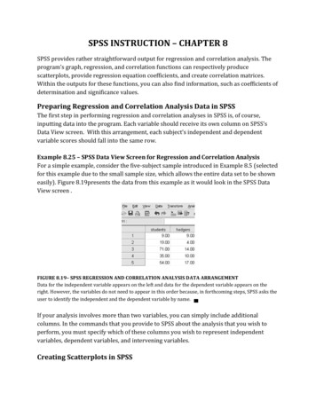
SPSS INSTRUCTION – CHAPTER 8SPSS provides rather straightforward output for regression and correlation analysis. Theprogram’s graph, regression, and correlation functions can respectively producescatterplots, provide regression equation coefficients, and create correlation matrices.Within the outputs for these functions, you can also find information, such as coefficients ofdetermination and significance values.Preparing Regression and Correlation Analysis Data in SPSSThe first step in performing regression and correlation analyses in SPSS is, of course,inputting data into the program. Each variable should receive its own column on SPSS’sData View screen. With this arrangement, each subject’s independent and dependentvariable scores should fall into the same row.Example 8.25 – SPSS Data View Screen for Regression and Correlation AnalysisFor a simple example, consider the five-subject sample introduced in Example 8.5 (selectedfor this example due to the small sample size, which allows the entire data set to be showneasily). Figure 8.19presents the data from this example as it would look in the SPSS DataView screen .FIGURE 8.19– SPSS REGRESSION AND CORRELATION ANALYSIS DATA ARRANGEMENTData for the independent variable appears on the left and data for the dependent variable appears on theright. However, the variables do not need to appear in this order because, in forthcoming steps, SPSS asks theuser to identify the independent and the dependent variable by name. If your analysis involves more than two variables, you can simply include additionalcolumns. In the commands that you provide to SPSS about the analysis that you wish toperform, you must specify which of these columns you wish to represent independentvariables, dependent variables, and intervening variables.Creating Scatterplots in SPSS
Basic scatterplots are most easily created through SPSS’s Graphs function. SPSSinstructions forChapter 2 and Chapter 3 explain how to use this function to create bargraphs, pie charts, and frequency histograms. The process for creating scatterplots in SPSSbegins the same way.1. From the pull-down menu under the Graphs option at the top of the data view orvariable view screen, select “Legacy Dialogues.” A listing of graphs and charts availablethrough this method should appear.2. Select “Scatter/Dot.” A window entitled Scatter/Dot should appear. The Scatter/Dotwindow contains various options for the graph. A two-variable situation requires aSimple Scatter. A three-variable situation, such as that described in Section 8.3.1,requires a 3-D Scatter. After selecting the name of the appropriate scatterplot, click“Define.”a. For a simple scatterplot, a new window, entitled Simple Scatterplot should appear.FIGURE 8.20 – SPSS SIMPLE SCATTERPLOT WINDOWThe user creates two-variable scatterplot by identifying the independent (X) and dependent (Y)variables from those listed on the left side of the window. To do so, highlight the name of eachvariable and click on the arrow next to the box labeled with the appropriate axis name.Identify the independent variable by moving its name from the box on the left to thebox labeled “X Axis.” Identify the dependent variable by moving its name from thebox on the left to the box labeled “Y Axis.”b. For a 3-D scatterplot, a new window, entitled, 3-D Scatterplot should appear.
FIGURE 8.21 – SPSS 3-D SCATTERPLOT WINDOWThe user creates three-variable scatterplot by identifying the two independent variables and thedependent variable from those listed on the left side of the window. To do so, highlight the name ofeach variable and click on the arrow next to the box labeled with the appropriate axis name.Move the names of each of the two independent variables and the dependentvariable from the box on the left to a box on the right marked for one of the axis. Theassignment of the three variables to the X, Y, and Z axis on the graph depends uponthe user’s intentions and preference for the graph’s appearance.3. Click OK.Example 8.26 – Simple Scatterplot in SPSSThe steps for producing a simple scatterplot can be applied to the examples from Section8.2.1. The following graph results from moving the name of the independent variable,students, to the box labeled, “X Axis,” and moving the name of the dependent variable,“hedgers,” to the box labeled “Y Axis.”
FIGURE 8.22 – SPSS SIMPLE SCATTERPLOT OUTPUTThe scale for independent-variable scores lies along the X axis and the scale for dependent-variable scoreslies along the Y axis. Each point represents a particular independent and dependent variable score.This particular scatterplot indicates that, as class size increases, teachers’ use of hedgerstends to increase. Thus, it suggests a positively-sloped regression line. The basic SPSS scatterplot does not show the regression line. If you would like the graph toinclude this line, you must use SPSS’s Chart Editor. To access the Chart Editor, you mustdouble click on the scatterplot.The Chart Editor refers to the least-squares regression line as a fit line. The pull-downmenu for the Elements function in the Chart Editor contains a “Fit Line at Total” option.(Often, the lowest menu bar in the Chart Editor also contains a shortcut icon for thisprocess.) Selecting this option begins the process for overlaying the regression line ontothe existing scatterplot.1. From the “Elements” pull-down menu in the Chart Editor, select “Fit Line at Total.”2. A new window entitled Properties should appear.
FIGURE 8.23 – SPSS CHART EDITOR PROPERTIES WINDOWThe choice of a fit method determines the line or curve that SPSS superimposes on the scatterplot. Simpleanalyses may require only a horizontal line to visually indicate the mean of all Y values. A linear fitproduces a least-squares regression line. Loess, quadratic, and cubic fits refer to curvilinear relationships.Select the appropriate Fit Method from the options provided. Most analyses require alinear fit. However, if you wish to investigate a possible curvilinear relationship, youmay wish to request a cubic, quadratic, or loess fit.3. Click CLOSE.Example 8.27 – Regression Line in SPSSFigure 8.23 shows the scatterplot in Figure 8.22 with an added regression line, obtained byrequesting a linear fit within the Chart Editor window. As expected, the line has a positiveslope.
FIGURE 8.24 – SPSS SIMPLE SCATTERPLOT WITH REGRESSION LINE OUTPUTThe regression line indicates the general linear trend of points. This particular line is the one that SPSSidentifies as producing the smallest sum of squared residuals for all points on the scatterplot.In this case, the points may fit a curvilinear path, particularly a cubic curve, slightly betterthan they fit a linear path. Requesting a cubic fit in the Chart Editor window producesFigure 8.26.
FIGURE 8.26 – SPSS SIMPLE SCATTERPLOT WITH CUBIC CURVE OUTPUTThe curve that appears in Figure 8.26 indicates the general cubic trend of points. This particular cubic curveis the one SPSS identifies as producing the smallest sum of squared residuals for all points on the scatterplot.This curve does, in fact, seem to fit the data better than Figure 8.25’s line does. Theresearcher may, therefore, which to characterize the relationship between the number ofstudents in a class and the number of hedgers used per hour by the teacher as curvilinear. Example 8.28 – 3-D Scatterplot in SPSSA three-dimensional scatterplot can represent the two variables from Example 8.26 andExample 8.27 along with the questions/hour variable used to demonstrate calculation ofthe multiple correlation coefficient in Example 8.13 In Example 8.13, x corresponds to thenumber of students in a particular class, y corresponds to the number of hedgers used perhour by the teacher, and z corresponds to the number of student questions per hour.Assigning these three variables to the appropriate axes in the 3-D Scatterplot windowproduces the following scatterplot.FIGURE 8.25 – SPSS 3-D SCATTERPLOT OUTPUTScales for the two independent variables appear along the X axis and the Y axis. The scale for the dependentvariable appears along the Z axis. The researcher, however, can assign the variables to the axes that suit his orher purposes. Each point represents a particular subject’s scores for the two independent variables and thedependent variable.
The points on this scatterplot seem to float in space. Actually, though, each point is situatedat the intersection of the planes representing the enrollment for a particular class, thenumber of hedgers used per hour by the teacher of that class and the number of questionsasked per hour by students in the class. You should know that methods of creating a scatterplot in SPSS other than “LegacyDialogues” option exist. The “Chart Builder” function within the “Graph” menu, forinstance, also leads you through steps that produce a scatterplot. With the Chart Builder,you gain some more control over the appearance and components of the scatterplot thanyou have when using Legacy Dialogues. However, when comparing the two methods, theprocess needed to use the Chart Builder is a bit more complicated.If you need to create a scatterplot that uses data points other than raw values you may wishto use a different approach. SPSS’s regression analysis function allows you to create suchscatterplots. By clicking on the window’s “plots” button, you can access a new, entitled,Linear Regression: Plots, which allows you to specify scales based upon standardizedvalues, residuals, and predicted values. This function generally has the most value forsomewhat advanced analyses.Regression Analysis in SPSSWith the exception of the scatterplot, itself, you can obtain all pairwise regression andcorrelation values by using SPSS’s “Regression” function. Output from the following stepsincludes regression equation coefficients, r, and r2.1. Select “Regression” from SPSS’s Analyze pull-down menu and then, assuming a linearregression is desired, select the “Linear” option.2. A window entitled Linear Regression should appear. A box in the upper left of thewindow contains the names of all variables.
FIGURE 8.26 – SPSS LINEAR REGRESSION WINDOWThe user obtains regression values by identifying the independent variable(s) and the dependent variablefrom those listed on the left side of the window. To do so, highlight the name of the variable and click onthe arrow next to the appropriate box.Move the names of the independent and dependent variables to the properly-labeledboxes on the right. If the user moves the name of only one variable the box labeled“independent variable(s)”, SPSS performs a bivariate regression analysis. If the namesof more than one variable are moved to the “independent variable(s) box, SPSSperforms a multiple regression analysis.3. Click OKFour output tables result. The first of these tables simply identifies the variables used forthe analysis. The other three tables provide the information that you need to assess therelationship between the independent and dependent variables. You can find thecorrelation coefficient and the coefficient of determination in the Model Summary table andcoefficients for the regression equation in the Coefficients table’s column “B.” SPSS refersto the y-intercept as the constant and lists each slope next to its corresponding variable’sname.The other table included in SPSS output provides ANOVA results. As explained in Section8.6, some statisticians supplement regression and correlation analysis with an ANOVA.Although a regression and correlation analysis addresses the trend in changes betweenindependent and dependent variable scores, it does not measure the sizes of differencesbetween scores on either factor. So, even if a trend exists, differences in dependent-variablescores associated with changes in independent-variable scores may be so miniscule thatthe trend becomes negligible. Those concerned about this issue may use an ANOVA
determine whether significant differences exist between dependent-variable scores. Whenconducting an ANOVA in this circumstance, SPSS regards the independent variable as acategorical measure. Each independent-variable score, thus, defines a separate category,often resulting in categories that contain only one subject. Then, the ANOVA compares thedependent-variable score that corresponds to each independent-variable category. You caninterpret the results of this test just as you would interpret the results of any ANOVA.(Please see Chapter 7 for information about ANOVAs.)Example 8.29 – SPSS Regression OutputTo further understand how to locate and interpret relevant regression and correlationcoefficients, consider the four output tables as they apply to the bivariate situation used forExample 8.26 and Example 8.27.Variables ovedMethodstudentsa. Entera. All requested variables entered.b. Dependent Variable: hedgersModel SummaryModel1RAdjusted RStd. Error of theSquareEstimateR Square.703a.494.4812.59045a. Predictors: (Constant), studentsANOVAbSum ofModel1SquaresdfMean 710Total504.40039a. Predictors: (Constant), studentsb. Dependent Variable: hedgersF37.167Sig.000a
icientsCoefficientsB(Constant)Std. 116.096.000a. Dependent Variable: hedgersTABLE 8.9, TABLE 8.10, TABLE 8.11, AND TABLE 8.12 – SPSS LINEAR REGRESSION OUTPUTSPSS output for the linear regression command includes four tables. Table 8.9, entitled “VariablesEntered/Removed,” indicates the independent variables and footnotes the name of the dependent variable.Table 8.10, Table 11, and Table 8.12 provide information about the changes in variable scores. Thecorrelation coefficient (r) and the coefficient of determination (r2) found in the Model Summary, indicate thestrength of the linear trend between the variables. The significance value in the ANOVA table, when comparedto a predetermined α, indicates whether changes in dependent- variable scores that accompany changes inindependent variable scores are significant. Finally, the Coefficients table provides the y-intercept and theslope for the regression equation.The correlation coefficient of .703, from Table 8.10, suggests that the number of students ina class and number of hedgers used per hour by the teacher have a strong (although barelyso) linear relationship. For those who do not wish to square the correlation coefficientthemselves, this table also includes the coefficient of determination, which indicates thatdifferences in the number of student in the class can explain 49.4% of differences inteachers’ use of hedgers. Further, the ANOVA produces a p-value of .000, which, obviously,lies below all α values. So, one could conclude that the number of hedgers used by teachersper hour changes significantly with respect to in the number of students in the class. Theregression equation helps to further describe this change. Using the regression equation ofy 1.017 .101x, obtained from value in Table 8.12, one can the dependent-variable scorefor each independent-variable score. Each x value substituted into the equation and the yvalue that results provides an ordered pair that falls on the regression line. This processproduces a best guess for the number of hedgers used based upon class size. If you input more than one variable name into the Linear Regression window’s“Independent Variable(s)” box, output looks similar to that shown in Example 8.29. In thiscase, however, the Model Summary provides the multiple correlation coefficient and thecoefficient of multiple determination. Also, the “B” column in the Coefficients table includesa slope for each independent variable.Correlation Matrices in SPSS
You may not always want to obtain all of the information provided by SPSS’s regressionanalysis. In some situations, correlation coefficients, alone, suffice. The Correlate functioncan not only provide these values without unneeded regression output, but can also displaycoefficients for more than one pair of variables at a time and can compute partialcorrelation coefficients. Coefficients appear in a correlation matrix. The following stepsproduce this output.1. Select “Correlate” from SPSS’s Analyze pull-down menu. Then, indicate whether SPSSshould calculate bivariate (pairwise) or partial correlation coefficients.2. a. For a bivariate analysis, a new window entitled Bivariate Correlations, shouldappear.FIGURE 8.27 – SPSS BIVARIATE CORRELATIONS WINDOWSPSS calculates correlation coefficients between each pair of variables with names appearing in thebox labeled “Variables.” The user should move the name of each variable involved in the analysisfrom the box on the left of the window by highlighting the name of the variable and clicking on thearrow to the left of the “Variables” box.Move the name of all variables that you would like to analyze from the list ofvariables on the left of the window to the box labeled “Variables.” The “Variables”box can contain as many variable names as needed. SPSS will calculate the pairwisecorrelation coefficient between each pair of variables listed. For instance, if thenames of variables “x”, “y”, and “z” appear in the “Variable” box, SPSS calculates rXY,rXZ, and rYZ.b. For partial correlations, a new window entitled, Partial Correlations, should appear.
FIGURE 8.28 – SPSS PARTIAL CORRELATIONS WINDOWSPSS calculates correlation coefficients between each pair of variables with names appearing in thebox labeled “Variables,” while removing the effects of any variables with names appearing in the boxlabeled “Controlling for.” The user should move the name of each variable involved in the analysisfrom the box on the left of the window by highlighting the name of the variable and clicking on thearrow to the left of the appropriate box.The names of intervening variables should be moved from the list of variable sonthe left of the window to the box labeled “Controlling for.” Move the name of thevariables involved in the correlation, itself, to the box labeled “Variables.”The “Variables” box can contain as many variable names as needed. SPSS willcalculate the correlation coefficient between each pair of variables listed whileholding steady the influence of the variable(s) appearing in the “Controlling for” box.3. Click OK.SPSS assigns each variable for which you requested a correlation to a row and column ofthe resulting correlation matrix. The coefficient for a particular linear relationship appearsat the intersection of each relevant row and column, as shown in Table 8.13, based upon ananalysis involving four variables, W, X, Y, and XZrYZrZZTABLE 8.13 - BASIC CORRELATION MATRIXThe interior portion of the table contains correlation coefficients for all pairs of variables. Values along thediagonal, which represent associations between each variable and itself, equal 1.00. This diagonal alsoserves as a line of symmetry because rWX rXW, rWY rYW, etc.
SPSS’s correlation matrix contains correlation coefficients as well as significance values andsample sizes for the data used to analyze each pair of variables.In some cases, your analysis may focus entirely upon these pairwise correlationcoefficients. Often, though, obtain these values is just the first step in a multiple regressionor correlation analysis.Example 8.30 – SPSS Correlation MatrixOne may wish to begin an investigation into the relationship between class size, thenumber of hedgers used per hour by a teacher, and the number of questions asked per hourby students by considering pairwise correlation coefficients. These values appear in Table8.14.CorrelationsStudentsstudentsPearson Correlation1.000hedgersPearson CorrelationSig. (2-tailed)NquestionsPearson CorrelationSig. **1.000.495**Sig. 000.001404040TABLE 8.14 - SPSS PAIRWISE CORRELATION MATRIXThe correlation coefficient for each pair of variables appears at the intersection of one variable’s row and theother variable’s column. Each variable correlates perfectly with itself, as evidenced by the coefficients of 1.00 at the intersection of a particular variables’ row and column.The number of students in a class correlates strongly with the number of hedgers used perhour by the teacher of that class (rXY .703). A moderate correlation exists between thenumber or students in a class and the number of questions asked per hour by students (rXZ .592) as well as between the number of questions asked per hour by students and thenumber of hedgers used per hour by the teacher (rYZ .495). The fact that all of thesecorrelation coefficients have positive values indicates that increases in one variablecorrespond to increases in the other.
A table similar to Table 8.14 emerges from SPSS when you request partial correlationcoefficients. In this case, SPSS informs the user that it has held constant the impact ofintervening variables by including their names under a “control variable” heading in theoutput.Example 8.31 – SPSS Partial Correlation MatrixTable 8.15 shows the SPPS results comparable to the calculations in Example 8.16. Thecorrelation matrix values describe the relationship between the number of questions askedper hour by students and the number of hedgers used per hour by the teacher researcherasks SPSS, independent of any influence of the percentage of factual information in coursematerial.CorrelationsControl tionHedgers1.000.628Significance (2-tailed).372Df02Correlation.6281.000Significance (2-tailed).372.20DfTABLE 8.15 - SPSS PARTIAL CORRELATION MATRIXBy listing “factualinfo” as a control variable on the left side of the table, SPSS reminds the user that it removedany influence that the percentage of factual information in a course has upon the number of students in theclass and the number of hedgers used per hour by the teacher.Because it plays the role of an intervening variable, “factual” is identified as a controlvariable in Table 8.15 rather than appearing as part of the main correlation matrix. Theresulting partial correlation coefficient of .628 also emerged from the calculations inExample 8.16. This value indicates a moderate tendency for the number of hedgers used bythe teacher to increase as class enrollment increases when discounting the effects of theintervening variable upon both of the other two variables. The “Linear Regression” box provides another method for obtaining partial correlations.Although this method only displays one partial correlation coefficient at a time, it alsoprovides part correlation coefficients, which you cannot obtain in matrix form. If you need
to include part correlation coefficients in your analysis, therefore, you may prefer followingprocedure.1. Select “Regression” from SPSS’s Analyze pull-down menu. Then, select the “Linear”option.2. A window entitled Linear Regression should appear. Follow the procedure describedearlier in this document for identifying the independent variable(s) and dependentvariable for the analysis. However, include the intervening variable(s) among those onthe independent variable list. Be sure to remember which of the variables is the trueindependent variable and which are intervening variables.3. Click on the button marked, “Statistics,” on the right of the Linear Regression window. Anew window, entitled, Linear Regression: Statistics should appear.FIGURE 8.29 – LINEAR REGRESSION: STATISTICS WINDOWThe prompt for part and partial correlations can be found in this window. With this option selected, SPSScalculates correlation coefficients between one independent variable and the dependent variable,independent of all other independent variables identified in the Linear Regression window.4. Mark the box labeled “Part and partial correlations,” located on the right side of thewindow. Doing so tells SPSS to calculate the correlation between the dependentvariable and each independent variable while holding constant the effects of all otherindependent variables.5. Click “Continue” to return to the Linear Regression window.6. Click OK.The partial and part correlation coefficients appear in the output’s “Coefficients” table,under the heading “Correlations.”
Example 8.32 – SPSS Part and Partial Correlation OutputTable 8.16 includes the partial correlation coefficient first presented in Example 8.31 aswell as the comparable part correlation rdizedCoefficientsCoefficientsB(Constant)Std. 3-.002a. Dependent Variable: hedgersTABLE 8.16 – SPSS COEFFICIENTS TABLE WITH PARTIAL AND PART CORRELATIONSPartial and part correlation coefficients appear on the far right of the table. The values in the row labeled,“students” pertain to the relationship between the number of students in the course and the number ofhedgers used per hour by the teacher independent of the amount of factual information in the course. Thetable also provides coefficients for the multiple regression equation that uses the number of students and thepercentage of factual information in a course to predict the number of hedgers used per hour by the teacher.Not surprisingly, Table 8.16 and the correlation matrix in Example 8.32 both identify thepartial correlation as .628. One would rely upon Table 8.16, however, to learn the partcorrelation coefficient. This value, .512, describes the linear relationship between thenumber of student in a class and the number of hedgers used by the teacher, independentof any effect that the amount of factual information in the class has upon the former. Thisvalue lies below both the pairwise and the partial correlation coefficients, but stillcharacterizes the relationship as moderately strong. Phi Analysis in SPSSThe request for a phi coefficient in SPSS takes place within the Crosstabulations context. Toaccess this window and to instruct SPSS to include the phi-coefficient along with itscrosstabulation output, you should use the following steps.1. Select “Descriptive Statistics” from SPSS’s Analyze pull-down menu.2. A new menu, containing a “Crosstabs” option appears. Select this option.3. A Crosstabs window should appear.
FIGURE 8.30 – SPSS CROSSTABS WINDOWThe user should move the name of one variable from the box on the left of the window to the box labeled“Row(s)” and the name of another variable from the box on the left to the box labeled “Colunm(s).”Highlighting the name of the variable and clicking on the arrow to the left of the “Row(s)” or “Column(s)”box moves the variable name to the appropriate place.Move the name of one variable involved in the analysis from the list on the left of thewindow to the “Row(s)” box. Move the name of the other variable involved in theanalysis from the list on the left of the window to the “Column(s)” box.4. Click the “Statistics” button, located on the right of the window. A new window entitledCrosstabs: Statistics should appear.FIGURE 8.31 – SPSS CROSSTABS:STATISTICS WINDOW
The user instructs SPSS to include in its crosstabulation output by selecting the “Phi and Cramer’s V”option in the Crosstabs: Statitistics Window. The resulting value describes the trend in frequencies forcategories of the variables in the crosstabulation.Click on the open box next to the “Phi and Cramer’s V” listing. Be sure that this boxcontains a check mark.5. Click the “Continue” button at the bottom of the page. You should return to theCrosstabs window.6. Click OK.The output that results from these steps consists of a crosstabulation table (discussed inChatper 2) and a Symmetric Measures table. The second of these contains the phicoefficient.Example 8.33 – SPSS Crosstabulation Output Including Symmetric MeasuresThe output for a crosstabulation and phi analysis involving the student enrollmentcategories and the hedger use categories introduced in Section 8.4 of the chapter appearsas follows.Case Processing SummaryCasesValidNstudcats * ercent40studcats * hedgecats CrosstabulationCounthedgecatsless than 5Studcatsfewer than 3030 or moreTotal5 or moreTotal1321542125172340Symmetric MeasuresValueApprox. Sig.100.0%
Nominal by NominalPhi.692.000Cramer's V.692.000N of Valid Cases40TABLE 8.17, TABLE 8.18, and TABLE 8.19 – SPSS CROSSTABULATION AND PHI COEFFICIENT OUTPUTTable 8.6 and 8.7 are part of SPSS’s standard crosstabulation output. The value of that appears in theSymmetric Measures table indicates the strength of the trend in frequencies of classes that fall into the twoenrollment and the two hedgers categories.Table 8.19’s phi coefficient of .692 indicates a moderate (close to strong) trend of largervalues in the upper left and lower right cells than in the other two cells of the Table 8.18’scrosstabulation.
SPSS INSTRUCTION – CHAPTER 8 SPSS provides rather straightforward output for regression and correlation analysis. The program’s graph, regression, and correlation functions can respectively produce scat