Transcription
Engineering AnalysisWith ANSYS Software
This page intentionally left blank
Engineering AnalysisWith ANSYS SoftwareY. Nakasone and S. YoshimotoDepartment of Mechanical EngineeringTokyo University of Science, Tokyo, JapanT. A. StolarskiDepartment of Mechanical EngineeringSchool of Engineering and DesignBrunel University, Middlesex, UKAMSTERDAM BOSTON HEIDELBERG LONDON NEW YORK OXFORDPARIS SAN DIEGO SAN FRANCISCO SINGAPORE SYDNEY TOKYOButterworth-Heinemann is an imprint of Elsevier
Elsevier Butterworth-HeinemannLinacre House, Jordan Hill, Oxford OX2 8DP30 Corporate Drive, Burlington, MA 01803First published 2006Copyright 2006 N. Nakasone, T. A. Stolarski and S. Yoshimoto. All rights reservedThe right of Howard D. Curtis to be identified as the author ofthis work has been asserted in accordance with the Copyright, Design andPatents Act 1988No part of this publication may be reproduced in any material form (includingphotocopying or storing in any medium by electronic means and whether ornot transiently or incidentally to some other use of this publication) withoutthe written permission of the copyright holder except in accordance with theprovisions of the Copyright, Designs and Patents Act 1988 or under the terms of alicence issued by the Copyright Licensing Agency Ltd, 90 Tottenham Court Road,London, England W1T 4LP. Applications for the copyright holder’s writtenpermission to reproduce any part of this publication should be addressed tothe publisherPermissions may be sought directly from Elsevier’s Science & TechnologyRights Department in Oxford, UK: phone ( 44) 1865 843830,fax: ( 44) 1865 853333, e-mail: permissions@elsevier.co.uk.You may also complete your request on-line via the Elsevier homepage(http://www.elsevier.com), by selecting ‘Customer Support’ and then‘Obtaining Permissions’The copyrighted screen shots of the ANSYS software graphical interface thatappear throughout this book are used with permission of ANSYS, Inc.ANSYS and any and all ANSYS, Inc. brand, product, service and feature names,logos and slogans are registered trademarks or trademarks of ANSYS, Inc. orits subsidiaries in the United States or other countries.British Library Cataloguing in Publication DataA catalogue record for this book is available from the British LibraryLibrary of Congress Cataloguing in Publication DataA catalogue record for this book is available from the Library of CongressISBN 0 7506 6875 XFor information on all Elsevier Butterworth-Heinemannpublications visit our website at http://books.elsevier.comTypeset by Charon Tec Ltd (A Macmillan Company), Chennai, Indiawww.charontec.comPrinted and bound by MPG Books Ltd., Bodmin, Cornwall
ContentsPrefaceThe aims and scope of the bookxiiixvChapter1Basics of finite-element method1.1Method of weighted residuals1.1.11.1.21.21.3Rayleigh–Ritz methodFinite-element method1.3.11.3.21.4Sub-domain method (Finite volume method)Galerkin methodOne-element caseThree-element caseFEM in two-dimensional elastostatic problems1.4.11.4.21.4.31.4.4Elements of finite-element procedures in the analysis ofplane elastostatic problemsFundamental formulae in plane elastostatic problems1.4.2.1 Equations of equilibrium1.4.2.2 Strain–displacement relations1.4.2.3 Stress–strain relations (constitutive equations)1.4.2.4 Boundary conditionsVariational formulae in elastostatic problems: the principleof virtual workFormulation of the fundamental finite-element equationsin plane elastostatic problems1.4.4.1 Strain–displacement matrix or [B] matrix1.4.4.2 Stress–strain matrix or [D] matrix1.4.4.3 Element stiffness equations1.4.4.4 Global stiffness equations1.4.4.5 Example: Finite-element calculations for a squareplate subjected to uniaxial uniform 525273034v
vi ContentsChapter2Overview of ANSYS structure and visualcapabilities2.12.2IntroductionStarting the ving and restoring jobsOrganization of filesPrinting and plottingExiting the programPreprocessing stage2.3.1Building a modelDefining element types and real constantsDefining material propertiesConstruction of the model2.3.2.1 Creating the model geometry2.3.2.2 Applying loads2.3.1.12.3.1.22.3.22.42.5Solution stagePostprocessing lication of ANSYS to stress analysis513.1515253Cantilever beam3.1.13.1.23.1.33.1.43.1.5Example problem: A cantilever beamProblem description3.1.2.1 Review of the solutions obtained by theelementary beam theoryAnalytical procedures3.1.3.1 Creation of an analytical model3.1.3.2 Input of the elastic properties of the beammaterial3.1.3.3 Finite-element discretization of the beam area3.1.3.4 Input of boundary conditions3.1.3.5 Solution procedures3.1.3.6 Graphical representation of the resultsComparison of FEM results with experimental onesProblems to solveAppendix: Procedures for creating stepped beamsA3.1Creation of a stepped beamHow to cancel the selection of areasCreation of a stepped beam with a rounded filletA3.2.1 How to display area numbersA3.1.1A3.2535353565762717376768080818184
Contents3.2The principle of St. Venant3.2.13.2.23.2.33.2.43.3Stress concentration due to elliptic holes3.3.13.3.23.3.33.3.43.3.53.4Example problem: An elastic plate with an elliptic hole inits center subjected to uniform longitudinal tensile stress σoat one end and damped at the other endProblem descriptionAnalytical procedures3.3.3.1 Creation of an analytical model3.3.3.2 Input of the elastic properties of the platematerial3.3.3.3 Finite-element discretization of the quarterplate area3.3.3.4 Input of boundary conditions3.3.3.5 Solution procedures3.3.3.6 Contour plot of stress3.3.3.7 Observation of the variation of the longitudinalstress distribution in the ligament regionDiscussionProblems to solveStress singularity problem3.4.13.4.23.4.33.4.43.4.53.5Example problem: An elastic strip subjected to distributeduniaxial tensile stress or negative pressure at one endand clamped at the other endProblem descriptionAnalytical procedures3.2.3.1 Creation of an analytical model3.2.3.2 Input of the elastic properties of the strip material3.2.3.3 Finite-element discretization of the strip area3.2.3.4 Input of boundary conditions3.2.3.5 Solution procedures3.2.3.6 Contour plot of stressDiscussionExample problem: An elastic plate with a crack of length 2ain its center subjected to uniform longitudinal tensile stressσ0 at one end and clamped at the other endProblem descriptionAnalytical procedures3.4.3.1 Creation of an analytical model3.4.3.2 Input of the elastic properties of the platematerial3.4.3.3 Finite-element discretization of the centercracked tension plate area3.4.3.4 Input of boundary conditions3.4.3.5 Solution procedures3.4.3.6 Contour plot of stressDiscussionProblems to solveTwo-dimensional contact 0
viii Contents3.5.13.5.23.5.33.5.43.5.5Example problem: An elastic cylinder with a radius of length(a) pressed against a flat surface of a linearly elastic mediumby a force Problem descriptionAnalytical procedures3.5.3.1 Creation of an analytical model3.5.3.2 Input of the elastic properties of the material forthe cylinder and the flat plate3.5.3.3 Finite-element discretization of the cylinder andthe flat plate areas3.5.3.4 Input of boundary conditions3.5.3.5 Solution procedures3.5.3.6 Contour plot of stressDiscussionProblems to 1Chapter4Mode analysis4.14.2IntroductionMode analysis of a straight bar4.2.14.2.24.2.34.2.44.2.54.3Problem descriptionAnalytical solutionModel for finite-element analysis4.2.3.1 Element type selection4.2.3.2 Real constants for beam element4.2.3.3 Material properties4.2.3.4 Create keypoints4.2.3.5 Create a line for beam element4.2.3.6 Create mesh in a line4.2.3.7 Boundary conditionsExecution of the analysis4.2.4.1 Definition of the type of analysis4.2.4.2 Execute calculationPostprocessing4.2.5.1 Read the calculated results of the first mode ofvibration4.2.5.2 Plot the calculated results4.2.5.3 Read the calculated results of the second and thirdmodes of vibrationMode analysis of a suspension for hard-disc drive4.3.14.3.2Problem descriptionCreate a model for analysis4.3.2.1 Element type selection4.3.2.2 Real constants for beam element4.3.2.3 Material 57157159161161161161163163163163165168
eate keypointsCreate areas for suspensionBoolean operationCreate mesh in areasBoundary conditionsAnalysis4.3.3.14.3.3.24.3.44.4Define the type of analysisExecute calculationPostprocessing4.3.4.1 Read the calculated results of the first mode ofvibration4.3.4.2 Plot the calculated results4.3.4.3 Read the calculated results of higher modes ofvibrationMode analysis of a one-axis precision moving tableusing elastic hinges4.4.14.4.24.4.34.4.4Problem descriptionCreate a model for analysis4.4.2.1 Select element type4.4.2.2 Material properties4.4.2.3 Create keypoints4.4.2.4 Create areas for the table4.4.2.5 Create mesh in areas4.4.2.6 Boundary conditionsAnalysis4.4.3.1 Define the type of analysis4.4.3.2 Execute calculationPostprocessing4.4.4.1 Read the calculated results of the first mode ofvibration4.4.4.2 Plot the calculated results4.4.4.3 Read the calculated results of the second and thirdmodes of vibration4.4.4.4 Animate the vibration mode r5Analysis for fluid dynamics5.15.2IntroductionAnalysis of flow structure in a diffuser5.2.15.2.2Problem descriptionCreate a model for analysis5.2.2.1 Select kind of analysis5.2.2.2 Element type selection5.2.2.3 Create keypoints5.2.2.4 Create areas for diffuser215215216216216216217219221
x Contents5.2.2.55.2.2.65.2.35.2.45.2.55.3Create mesh in lines and areasBoundary conditionsExecution of the analysis5.2.3.1 FLOTRAN set upExecute calculationPostprocessing5.2.5.1 Read the calculated results of the first mode ofvibration5.2.5.2 Plot the calculated results5.2.5.3 Plot the calculated results by path operationAnalysis of flow structure in a channel with a butterflyvalve5.3.15.3.25.3.35.3.45.3.5Problem descriptionCreate a model for analysis5.3.2.1 Select kind of analysis5.3.2.2 Select element type5.3.2.3 Create keypoints5.3.2.4 Create areas for flow channel5.3.2.5 Subtract the valve area from the channel area5.3.2.6 Create mesh in lines and areas5.3.2.7 Boundary conditionsExecution of the analysis5.3.3.1 FLOTRAN set upExecute calculationPostprocessing5.3.5.1 Read the calculated results5.3.5.2 Plot the calculated results5.3.5.3 Detailed view of the calculated flow velocity5.3.5.4 Plot the calculated results by path plication of ANSYS to thermomechanics6.16.2General characteristic of heat transfer problemsHeat transfer through two walls6.2.16.2.26.2.36.2.46.3Steady-state thermal analysis of a pipe intersection6.3.16.3.26.3.36.3.46.3.56.4Problem descriptionConstruction of the modelSolutionPostprocessingDescription of the problemPreparation for model buildingConstruction of the modelSolutionPostprocessing stageHeat dissipation through ribbed surface263263265265265276280285285288291298306312
Contents6.4.16.4.26.4.36.4.4Problem descriptionConstruction of the pplication of ANSYS to contact betweenmachine elements7.17.2General characteristics of contact problemsExample problems7.2.1Pin-in-hole interference fitProblem descriptionConstruction of the modelMaterial properties and element typeMeshingCreation of contact pairSolutionPostprocessingConcave contact between cylinder and two blocks7.2.2.1 Problem description7.2.2.2 Model construction7.2.2.3 Material properties7.2.2.4 Meshing7.2.2.5 Creation of contact pair7.2.2.6 Solution7.2.2.7 PostprocessingWheel-on-rail line contact7.2.3.1 Problem description7.2.3.2 Model construction7.2.3.3 Properties of material7.2.3.4 Meshing7.2.3.5 Creation of contact pair7.2.3.6 Solution7.2.3.7 PostprocessingO-ring assembly7.2.4.1 Problem description7.2.4.2 Model construction7.2.4.3 Selection of materials7.2.4.4 Geometry of the assembly and meshing7.2.4.5 Creating contact interface7.2.4.6 Solution7.2.4.7 Postprocessing (first load step)7.2.4.8 Solution (second load step)7.2.4.9 Postprocessing (second load 01404410410412413423427436442444451453
This page intentionally left blank
PrefaceThis book is very much the result of a collaboration between the three co-authors:Professors Nakasone and Yoshimoto of Tokyo University of Science, Japan and Professor Stolarski of Brunel University, United Kingdom. This collaboration startedsome 10 years ago and initially covered only research topics of interest to the authors.Exchange of academic staff and research students have taken place and archive papershave been published. However, being academic does not mean research only. Theother important activity of any academic is to teach students on degree courses. Sincethe authors are involved in teaching students various aspects of finite engineeringanalyses using ANSYS it is only natural that the need for a textbook to aid studentsin solving problems with ANSYS has been identified.The ethos of the book was worked out during a number of discussion meetings andaims to assist in learning the use of ANSYS through examples taken from engineeringpractice. It is hoped that the book will meet its primary aim and provide practicalhelp to those who embark on the road leading to effective use of ANSYS in solvingengineering problems.Throughout the book, when we state “ANSYS”, we are referring to the structuralFEA capabilities of the various products available from ANSYS Inc. ANSYS is the original (and commonly used) name for the commercial products: ANSYS Mechanical orANSYS Multiphysics, both general-purpose finite element analysis (FEA) computeraided engineering (CAE) software tools developed by ANSYS, Inc. The companyactually develops a complete range of CAE products, but is perhaps best known forthe commercial products ANSYS Mechanical & ANSYS Multiphysics. For academicusers, ANSYS Inc. provides several noncommercial versions of ANSYS Multiphysicssuch as ANSYS University Advanced and ANSYS University Research.ANSYS Mechanical, ANSYS Multiphysics and the noncommercial variantscommonly used in academia are self-contained analysis tools incorporatingpre-processing (geometry creation, meshing), solver and post-processing modulesin a unified graphical user interface. These ANSYS Inc. products are general-purposefinite element modeling tools for numerically solving a wide variety of physics, suchas static/dynamic structural analysis (both linear and nonlinear), heat transfer, andfluid problems, as well as acoustic and electromagnetic problems.For more information on ANSYS products please visit the websitewww.ansys.com.J. NakasoneT. A. StolarskiS. YoshimotoTokyo, September 2006xiii
This page intentionally left blank
The aims andscope of the bookIt is true to say that in many instances the best way to learn complex behavior is bymeans of imitation. For instance, most of us learned to walk, talk, and throw a ballsolely by imitating the actions and speech of those around us. To a considerable extent,the same approach can be adopted to learn to use ANSYS software by imitation, usingthe examples provided in this book. This is the essence of the philosophy and theinnovative approach used in this book. The authors have attempted in this book toprovide a reader with a comprehensive cross section of analysis types in a variety ofengineering areas, in order to provide a broad choice of examples to be imitated inone’s own work. In developing these examples, the authors’ intent has been to exercisemany program features and refinements. By displaying these features in an assortmentof disciplines and analysis types, the authors hope to give readers the confidence toemploy these program enhancements in their own ANSYS applications.The primary aim of this book is to assist in learning the use of ANSYS softwarethrough examples taken from various areas of engineering. The content and treatmentof the subject matter are considered to be most appropriate for university studentsstudying engineering and practicing engineers who wish to learn the use of ANSYS.This book is exclusively structured around ANSYS, and no other finite-element (FE)software currently available is considered.This book is divided into seven chapters. Chapter 1 introduces the reader tofundamental concepts of FE method. In Chapter 2 an overview of ANSYS is presented.Chapter 3 deals with sample problems concerning stress analysis. Chapter 4 containsproblems from dynamics of machines area. Chapter 5 is devoted to fluid dynamicsproblems. Chapter 6 shows how to use ANSYS to solve problems typical for thermomechanics area. Finally, Chapter 7 outlines the approach, through example problems,to problems related to contact and surface mechanics.The authors are of the opinion that the planned book is very timely as there is aconsiderable demand, primarily from university engineering course, for a book whichcould be used to teach, in a practical way, ANSYS – a premiere FE analysis computerprogram. Also practising engineers are increasingly using ANSYS for computer-basedanalyses of various systems, hence the need for a book which they could use in aself-learning mode.The strategy used in this book, i.e. to enable readers to learn ANSYS by meansof imitation, is quite unique and very much different than that in other books whereANSYS is also involved.xv
This page intentionally left blank
Chapter1Basics offinite-elementmethodChapter outline1.1 Method of weighted residuals1.2 Rayleigh–Ritz method1.3 Finite-element method1.4 FEM in two-dimensional elastostatic problemsBibliography2571434arious phenomena treated in science and engineering are often described interms of differential equations formulated by using their continuum mechanicsmodels. Solving differential equations under various conditions such as boundary orinitial conditions leads to the understanding of the phenomena and can predict thefuture of the phenomena (determinism). Exact solutions for differential equations,however, are generally difficult to obtain. Numerical methods are adopted to obtainapproximate solutions for differential equations. Among these numerical methods,those which approximate continua with infinite degree of freedom by a discrete bodywith finite degree of freedom are called “discrete analysis.” Popular discrete analysesare the finite difference method, the method of weighted residuals, and the Rayleigh–Ritz method. Via these methods of discrete analysis, differential equations are reducedto simultaneous linear algebraic equations and thus can be solved numerically.This chapter will explain first the method of weighted residuals and the Rayleigh–Ritz method which furnish a basis for the finite-element method (FEM) by takingexamples of one-dimensional boundary-value problems, and then will compareV1
2 Chapter 1 Basics of finite-element methodthe results with those by the one-dimensional FEM in order to acquire a deeperunderstanding of the basis for the FEM.1.1Method of weighted residualsDifferential equations are generally formulated so as to be satisfied at any pointswhich belong to regions of interest. The method of weighted residuals determinesthe approximate solution ū to a differential equation such that the integral of theweighted error of the differential equation of the approximate function ū over theregion of interest is zero. In other words, this method determines the approximatesolution which satisfies the differential equation of interest on average over the regionof interest: L[u(x)] f (x) (a x b)(1.1)BC (Boundary Conditions): u(a) ua , u(b) ubwhere L is a linear differential operator, f (x) a function of x, and ua and ub the valuesof a function u(x) of interest at the endpoints, or the one-dimensional boundaries ofthe region D. Now, let us suppose an approximate solution to the function u beū(x) φ0 (x) n ai φi (x)(1.2)i 1where φi are called trial functions (i 1, 2, . . . , n) which are chosen arbitrarily asany function φ0 (x) and ai some parameters which are computed so as to obtain agood “fit.”The substitution of ū into Equation (1.1) makes the right-hand side non-zero butgives some error R:L[ū(x)] f (x) R(1.3)The method of weighted residuals determines ū such that the integral of the errorR over the region of interest weighted by arbitrary functions wi (i 1, 2, . . . , n) is zero,i.e., the coefficients ai in Equation (1.2) are determined so as to satisfy the followingequation: wi R dv 0(1.4)Dwhere D is the region considered.1.1.1Sub-domain method (finite volume method)The choice of the following weighting function brings about the sub-domain methodor finite-volume method. 1 (for x D)wi (x) (1.5)0 (for x / D)
1.1 Method of weighted residualsExample1.13Consider a boundary-value problem described by the following one-dimensionaldifferential equation: 2 d u u 0 (0 x 1)dx 2 BC: u(0) 0 u(1) 1(1.6)The linear operator L[·] and the function f (x) in Equation (1.6) are defined as follows:L[·] d2( · )dx 2f (x) u(x)(1.7)For simplicity, let us choose the power series of x as the trial functions φi , i.e.,ū(x) n 1 ci x i(1.8)i 0For satisfying the required boundary conditions,c0 0,n 1 ci 1(1.9)i 1so thatū(x) x n Ai (x i 1 x)(1.10)i 1If the second term of the right-hand side of Equation (1.10) is chosen as afirst-order approximate solutionū1 (x) x A1 (x 2 x)(1.11)the error or residual is obtained asR 10 wi R dx 1d 2 ū ū A1 x 2 (A1 1)x 2A1 0dx 21 A1 x 2 (A1 1)x 2A1 dx 0113A1 062(1.12)(1.13)Consequently, the first-order approximate solution is obtained asū1 (x) x 3x(x 1)13(1.14)
4 Chapter 1 Basics of finite-element method(Example 1.1continued)which agrees well with the exact solutionu(x) e x e xe e 1(1.15)as shown by the dotted and the solid lines in Figure 1.1.1Exact solutionSub-domain methodGalerkin methodRayleigh–Ritz methodFinite element method0.80.6u0.40.2000.20.40.60.81xFigure 1.11.1.2Comparison of the results obtained by various kinds of discrete analyses.Galerkin methodWhen the weighting function wi in Equation (1.4) is chosen equal to the trial functionφi , the method is called the Galerkin method, i.e.,wi (x) φi (x) (i 1, 2, . . . , n)(1.16)and thus Equation (1.4) is changed to φi R dv 0(1.17)DThis method determines the coefficients ai by directly using Equation (1.17) or byintegrating it by parts.Example1.2Let us solve the same boundary-value problem as described by Equation (1.6) in thepreceding Section 1.1.1 by the Galerkin method.The trial function φi is chosen as the weighting function wi in order to find thefirst-order approximate solution:w1 (x) φ1 (x) x(x 1)(1.18)
1.2 Rayleigh–Ritz method(Example 1.2continued)5Integrating Equation (1.4) by parts, 1 1wi R dx wi00d 2 ūd ū ū dx widx 2dx 1 1 00dwi d ūdx dx dx 1wi ū dx 00(1.19)is obtained. Choosing ū1 in Equation (1.11) as the approximate solution ū, thesubstitution of Equation (1.18) into (1.19) gives 1 φ1 R dx 010 1dφ1 d ūdx dx dx 1 1φ1 ū dx 0(2x 1)[1 A1 (2x 1)]dx0(x 2 x)[1 A1 (x 2 x)]dx 01A1A1 031230(1.20)Thus, the following approximate solution is obtained:ū1 (x) x 5x(x 1)22(1.21)Figure 1.1 shows that the approximate solution obtained by the Galerkin method alsoagrees well with the exact solution throughout the region of interest.1.2Rayleigh–Ritz methodWhen there exists the functional which is equivalent to a given differential equation,the Rayleigh–Ritz method can be used.Let us consider the example problem illustrated in Figure 1.2 where a particlehaving a mass of M slides from point P0 to lower point P1 along a curve in a verticalplane under the force of gravity. The time t that the particle needs for sliding fromthe points P0 to P1 varies with the shape of the curve denoted by y(x) which connectsthe two points. Namely, the time t can be considered as a kind of function t F[y]which is determined by a function y(x) of an independent variable x. The functionyP0My2(x)y3(x)y1(x)P1xFigure 1.2Particle M sliding from point P0 to lower point P1 under gravitational force.
6 Chapter 1 Basics of finite-element methodof a function F[y] is called a functional. The method for determining the maximumor the minimum of a given functional is called the variational method. In the caseof Figure 1.2, the method determines the shape of the curve y(x) which gives thepossible minimum time tmin in which the particle slides from P0 to P1 .The principle of the virtual work or the minimum potential energy in the field ofthe solid mechanics is one of the variational principles which guarantee the existenceof the function which makes the functional minimum or maximum. For unsteadythermal conductivity problems and viscous flow problems, no variational principlecan be established; in such a case, the method of weighting residuals can be adoptedinstead.Now, let [u] be the functional which is equivalent to the differential equation inEquation (1.1). The Rayleigh–Ritz method assumes that an approximate solution ū(x)of u(x) is a linear combination of trial functions φi as shown in the following equation:ū(x) n ai φi (x)(1.22)i 1where ai (i 1, 2, . . . , n) are arbitrary constants, φi are C 0 -class functions which havecontinuous first-order derivatives for a x b and are chosen such that the followingboundary conditions are satisfied:n ai φi (a) uai 1n ai φi (b) ub(1.23)i 1The approximate solution ū(x) in Equation (1.22) is the function which makes thefunctional [u] take stationary value and is called the admissible function.Next, integrating the functional after substituting Equation (1.22) into thefunctional, the constants ai are determined by the stationary conditions: 0 ai(i 1, 2, . . . , n)(1.24)The Rayleigh–Ritz method determines the approximate solution ū(x) by substitutingthe constants ai into Equation (1.22). It is generally understood to be a method whichdetermines the coefficients ai so as to make the distance between the approximatesolution ū(x) and the exact one u(x) minimum.Example1.3Let us solve again the boundary-value problem described by Equation (1.6) by theRayleigh–Ritz method. The functional equivalent to the first equation of Equation(1.6) is written as 1 1 du 2 1 2 [u] u dx(1.25)2 dx20Equation (1.25) is obtained by intuition, but Equation (1.25) is shown to really givethe functional of the first equation of Equation (1.6) as follows: first, let us takethe first variation of Equation (1.25) in order to obtain the stationary value of the
1.3 Finite-element methodequation: 1δ 07 du duδdx dx uδu dx(1.26)Then, integrating the above equation by parts, we have 1δ du dδudu uδu dx δudx dxdx0 01d2udx 2 1 010ddx duδu uδu dxdx u δu dx(1.27)For satisfying the stationary condition that δ 0, the rightmost-hand side ofEquation (1.27) should be identically zero over the interval considered (a x b),so thatd2u u 0(1.28)dx 2This is exactly the same as the first equation of Equation (1.6).Now, let us consider the following first-order approximate solution ū1 whichsatisfies the boundary conditions:ū1 (x) x a1 x(x 1)(1.29)Substitution of Equation (1.29) into (1.25) and integration of Equation (1.25)lead to 1 121112dx a1 a12x a1 (x 2 x) [ū1 ] [1 a1 (2x 1)]2 23 12230(1.30)Since the stationary condition for Equation (1.30) is written by 21 a1 0 a112 3(1.31)the first-order approximate solution can be obtained as follows:1ū1 (x) x x(x 1)8(1.32)Figure 1.1 shows that the approximate solution obtained by the Rayleigh–Ritzmethod agrees well with the exact solution throughout the region considered.1.3Finite-element methodThere are two ways for the formulation of the FEM: one is based on the directvariational method (such as the Rayleigh–Ritz method) and the other on the methodof weighted residuals (such as the Galerkin method). In the formulation based onthe variational method, the fundamental equations are derived from the stationaryconditions of the functional for the boundary-value problems. This formulationhas an advantage that the process of deriving functionals is not necessary, so it is
8 Chapter 1 Basics of finite-element methodeasy to formulate the FEM based on the method of the weighted residuals. In theformulation based on the variational method, however, it is generally difficult toderive the functional except for the case where the variational principles are alreadyestablished as in the case of the principle of the virtual work or the principle of theminimum potential energy in the field of the solid mechanics.This section will explain how to derive the fundamental equations for the FEMbased on the Galerkin method.Let us consider again the boundary-value problem stated by Equation (1.1): L[u(x)] f (x) (a x b)(1.33)BC (Boundary Conditions): u(a) ua u(b) ubFirst, divide the region of interest (a x b) into n subregions as illustrated inFigure 1.3. These subregions are called “elements” in the FEM.(e)N2e(e 1)(e 1)N1e 1N2e 11(e)N1ex1 ax2x3Element 1 Element 2Figure 1.3xexe 1xn 1 bElement e–1 Element e Element e 1Element nDiscretization of the domain to analyze by finite elements and their interpolation functions.Now, let us assume that an approximate solution ū of u can be expressed by apiecewise linear functio
FM-H6875.tex 28/11/2006 16: 7 page vi vi Contents Chapter2 Overview of ANSYS structure and visual capabilities 37 2.1 Introduction 37 2.2 Starting the program 38 2.2.1 Preliminaries 38 2.2.2 Saving and restoring jobs 40 2.2.3 Organization of files 41 2.2.4 Printing and plotting 42 2.2.5 Exiting the program 43 2.3 Preproces