Transcription
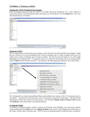
TUTORIAL 1: Welcome to ANSYS!Opening the ANSYS Workbench EnvironmentFrom the program menu list open the ANSYS 15.0 folder and select Workbench 15.0. Once ANSYS isactive and you have closed the popup window presented, you will be able to view the Project tab. This viewshould look like the view below.Setting the UNITSNow is a good time to set the units you are going to work with since the units typically do not change. Doingthis now will prevent you from modeling a bar 2 meters in diameter and 12 meters in length when you try tomodel a bar 2 inches in diameter and 12 inches in length. The first bar may fail under its own self-weightdepending on the material used! To change the units, or to check the units being used in an existing model,click on Units from the Project menu bar. You should see the following basic options for your unit system We will typically use either the predefined Metric units (default unit system) or the US Customary units inour models. At this point switch the units to the US Customary unit system by selecting it. The check markshould move to this Unit system in the menu shown. Also Switch to Display Values in Project Units insteadof as Defined, if this check mark is not already checked.Creating the ModelTo perform a structural analysis, which is what we are focusing on in Strengths, you will need to add thecorrect building block (system) from the Analysis Systems menu, which is the left-hand side (LHS) menu inthe Project window that is currently open. ANSYS can do an amazing number of different types of analyses,
including thermal, dynamic, buckling, fluid interaction, etc., but our focus is on Static Structural analysis,i.e., our systems are not moving and will only have static (unchanging) forces applied. This type of analysiswill allow us to determine the resulting displacements, stresses, strains, and internal forces/moments in anystructural component that are caused by loads that are assumed to vary slowly with respect to time. This isexactly the same type of results information we are looking for when we solve Strength of Materialsproblems by hand using theoretical and/or approximate methods.Click on the Static Structural item in the LHS menu, drag it into the Project Schematic window and thendrop it off specifically in the region defined by the green dashed box that appears. In a few seconds you willsee the following small window appear. This is the model system block.Typically you will give your system a new name that will allow you and others to pick this specific modelout of many others quickly in the future. To do this double click on the default name on the system andchange the name. For example you can rename the model YourName Axial Bar Tutorial.This process defines a specific system block that is made up of several components that are called cells.These cells define the sequential steps needed to perform the specific type of analysis. To perform youranalysis, you will work through the cells of each system in order—typically from top to bottom—defininginputs, specifying project parameters, running your simulation, and investigating the results. To interact withthe cells, you will typically do one of the following: Single-click: Single-click an object to select it. This does not modify data or initiate any action. Double-click: Double-click an object to initiate the default action, which may later help you increaseyour speed. Right- click: Right-click to display a context menu applicable to the current state of the selected object.Saving Your Model & any Future AnalysesBefore you go any further, save your current ANSYS workspace and system by selecting File- Save Asfrom the toolbar. Save your files to a folder that is on the desktop or to a folder on the CEE Scratch Drive.You can store files to a memory key also, but this may slow things done a little. As you continue through thedifferent program elements be sure to save your work from time to time in case anything bad happens andyou need to go back to a previous saved model. ANSYS does not have an Undo button so having previoussaved versions can be useful in helping you avoid starting from scratch if something goes wrong.Time to Start Modeling!To create a model in ANSYS and then analyze it you will work through the cells in the System menu in topto-bottom order. This means that you need to define the Engineering Data and Geometry before you can puttogether the Model, and you must have the Model defined before you can run the analysis and get theSolution and view the Results.To help you understand these cells and the process needed to create each one of the System Components wewill create a model of a solid, circular steel axial bar. The bar has a diameter of 1 inch, a length of 12 inches,
a concentrated load, P 10,000 lbf at one end and is fixed to a wall at the other end. This axial bar setup isshown in the picture below.To create the model we will need to define the material used – Steel; the geometry of the bar – length andcross-sectional shape and dimensions; the loading – force magnitude and direction; the boundary conditions– the type of support provided and the support locations; and the type of mesh element and the coarseness ofthe mesh used to analyze the system. A coarser mesh and simpler elements will provide less accurate resultsthan a more refined mesh and more complex elements, but the coarser mesh will provide quicker analysisresults as a tradeoff. The analysis part is straightforward once the model has been defined.Engineering DataTo have the correct behavior modeled, you need to define the type of material, along with its mechanicalproperties, using the Engineering Data cell. The model deformation response will depend on the materialdefined. To view the default Steel material properties, right-click on the Engineering Data cell and selectEdit You will see the following as the default. In some cases you will not see the bottom graph axes,which is just fine.Some of the numbers may look familiar, especially in this set of units, but we will set the material propertiesto reflect that we are using a standard A992 Steel material. The primary material properties that we need tospecify are the Modulus of Elasticity, E 29,000,000 psi and Poisson’s Ratio, ν 0.3. These will allow thecorrect relationship to exist between stress and strain in the model and when we run our hand calculations tocheck the results obtained. Other critical material properties that our analysis needs are the steel yieldstrength of 50,000 psi (50 ksi) and the steel ultimate strength of 65,000 psi (65 ksi). Although our bar willnot yield due to having a stress below the material yield stress, it is important to define these materialbehavior limits in case the stress is enough to cause yielding to occur. Yielding will lead to very largedeflections typically, so knowing if something has yielded becomes an important design consideration.These values are different from the default values provided by ANSYS and so you will need to change these.The A992 steel density is the same as the default ANSYS steel material and will be used in problems wherewe include the self-weight of the material as part of the loading.To change each value, click on each of the cells in the lower left pane and then enter the value desired in thebox that appear in the upper right pane. Remember the units are psi here. To change E and υ click on the sign in front of the Isotropic Elasticity menu item to open up its options. Then click on each cell to enter
29000000 for E and 0.3 for υ. Use the same process to change both the tensile and compressive yieldstrength to 50000 and the tensile and compressive ultimate strength to 65000.When you are done you should have the values shown in the screenshot below for our specific Steel material.Save the changes with Save. To return to the Project tab either close the A2: Engineering Data (X) tab orclick on the grayed-out Project tab to the left of the A2:engineering Data tab and leave the Engineering Data
tab open, but hidden. This action will take you back to the overall ANSYS project window.Engineering Data cell in your Axial Bar System menu should now have a green check mark next to it.TheGeometryDuring this semester, you will either create a new geometry from scratch using the DesignModeler programor you will import an existing geometry previously created by you or a colleague. We will jump right in andcreate our geometry for this axial bar model from scratch. To do this right click on the Geometry cell in theSystem menu and select New Geometry. This will open the DesignModeler program in a new window.This may take a little while depending on the computer you are working on but in the end you will see that anew window has been opened (with the green bullet and DM icon). This window should look like the onebelow.Note ‐ Sketching Tab & Modeling TabYou should notice that the LHS menu now presents a Tree Outline. The Tree Outline matches the logicalsequence of simulation steps. Object sub-branches relate to the main object. For example, an analysisenvironment object, such as Static Structural, will eventually contain loads. You can right-click on anobject to open a context menu that relates to that object. You can rename objects prior to and following thesolution process.Using the DesignModeler we will ‘draw’ our system part(s) using basic drawing tools and then extrude our2D cross-sections into 3D elements. To do this now, follow these steps: First, change the Units from the default of m to inch using the toolbar Units if you notice that the unitson the window scale are in shown in m instead of inch. Second, click on the YZ Plane leaf, which is located in the Tree Outline on the LHS, to have that planeavailable to draw on with a 2D shape. This will make the X axis the axial direction axis. Third, change the selection from the Modeling Tab showing the Tree Outline to the Sketching Tab thatallows drawing to begin.At this point you should see a set of Draw options listed in the LHS menu. The rest of the options includedin the Sketching Tab are hidden under the Modify, Dimension, Constraints, and Settings items.Draw Options under Sketching TabX‐axis is Axial Direction
Using the Draw options you will draw the bar circular cross-section. Click on the Circle draw command inthe LHS Draw menu. Using the mouse. hover over the axis origin and click to draw a circle shape. Drag themouse outward to create a circle in the XY plane. You do not need to worry at this point about the correctdiameter dimension.Once the circle is drawn we can input the correct the diameter dimension by changing to the DimensionsMenu from the Draw Menu on the LHS and clicking on the Diameter option. Click anywhere on your circleto define the D1 parameter location. When you do this an arrow defining the diameter will appear on yoursketch with the label D1. In the text box that appears on the LHS, type 1 in the D1 box and hit Enter todefine the circle’s actual diameter. Note that the circle dimension changes in the sketch to reflect this newvalue.Now select the function Extrude from the top tool bar. You will see a wireframe extrusion of the 2D crosssection into 3D in the x-axis direction in the Sketch.Change the FD1 value in LHS menu that appears showing the details of the Extrude1 to 12 inches and thenclick on the Apply button that is showing in the LHS. This will create a solid circular bar with this exact
extrusion length in your model. Now as a final step click to create the 3D bar element click on the Generateoption on the toolbar (it has the lightning bolt next to it). You should now have 3D cylindrical bar!You will find that you have been thrown out of the Sketching tab and back into the Modeling tab. This isfine. Before we move on, let’s rename some of the sketches and parts we have in the model. Click on the signs in the LHS tree menu to expand each one.Right-click on each label and rename the Sketch1 as CircularBarCrossSection and the Extruded Body Partcreated as AxialBar. For simple models this is not perhaps very useful; but with more complex models ithelps with searching to find what you want to work with. Keep the DesignModular program open but openthe ANSYS main window by clicking on the ANSYS icon (Black & Yellow A icon) along the bottomtoolbar.You should now see a nice green checkmark next to the Geometry cell in the System menu in the ANSYSProject window. As indicated, the Model cell is the next one that you will want to right-click on and selectEdit to work with. Another new window will open that is tagged with a red ball and giant M icon, whichstands for Mechanical. This Mechanical window will allow you to work on the meshing of the axial bar. Amesh is needed to run a Finite Element Analysis (FEA). The mesh takes the 3D axial bar part and representsit as many small elements that are connected by nodes. The FEA cannot run without having a mesh defined.
The LHS menu has changed to show the Model Components: Geometry, Mesh, Static Structural etc.The Mechanical Icon hides underneath the DesignModular Icon in the toolbarIn the Mechanical Tree Outline you should see a Mesh leaf. Right-click on Mesh and then select GenerateMesh. For now we will use the default mesh element. Later in the semester we will talk more about whathappens when you change the type of element or the size of the elements used to define the mesh. Once themesh is generated it will appear on the 3D bar as shown. The default ANSYS element type is officially a 3Dquadratic tetrahedron (solid) element. Typically you will not need to any other solid element.Sizing Options: Click on the to see the optionsIf you want to rotate the axial bar in space you can use any of the view buttons in the toolbar.Under the Sizing Menu Item on the LHS you can change the Sizing- Relevance Center from Coarse toMedium and the right-click on the Mesh leaf and click Update to see the mesh generated become morerefined, i.e., more elements are defined. Typically you would expect the Medium mesh to give better resultsthan the Coarse mesh, although it may take more time to do so. You can view what happens if you select theFine mesh option too.
Leave the model with the Medium mesh. If you go back to the ANSYS Project window you will now see agreen check mark next to the Model cell.Go back to the Mechanical window view. You can visually identify model parts based on a property of thatpart. For example, if an assembly is made of parts of different materials, you can color the parts based on thematerial. Click directly on the Geometry tree leaf in the Model window (not on the here but on theGeometry label) and under the Definition menu change the Display Style field to Material from BodyColor. The part colors are based on the material assignment. For example in a model with five parts wherethree parts use structural steel and two parts use aluminum, you will see the three structural steel parts in onecolor and the two aluminum parts in another color. The legend will indicate the color used along with thename of the material. In our case there is only one material color shown for structural steel in the legend.SetupUse the Setup cell to launch the appropriate application for that system. Using these options you will defineyour loads, boundary conditions, and otherwise configure your analysis in the application. Go back to theProject window and right-click on the Setup cell and select Edit You will work again in the sameMechanical model window but will need to right-click on the Static Structural leaf to access the functionsneeded. Many options will show when you select Insert as shown below.
For our current system we will Insert a Force to represent the axial load appliedat one end of the bar and Insert a Fixed Support to represent the fixed supportboundary condition at the other end of the bar.We will create the Force first. Right-click on Static Structural- Insert- Force. The first change to bemade is to change the Define by box selection from Vector to Components in the lower left menu. If youclick on this box you will be able to view the options using the arrow provided. The second change is to setthe magnitude of the X-direction force to be 10,000 lbs. If you notice that the force units are in N, you willneed to reset the units to inch and lb in the Mechanical window by selecting Units from the main toolbar.The positive X-axis direction will define the positive direction of the force in this case.So now the direction and magnitude of the load is defined, but we still need to define the location of the forceon the axial bar. Click on the X axis vector in the bottom right corner to change the view to look at the endview of the bar.
Then change the cursor to the select Face in the Toolbarand click on the end of the bar cross-section as near to the center of the cross-section as you can approximateto highlight this face of the bar. In the bottom left menu that shows the Details of “Force” click on theGeometry None Selected box that is highlighted in yellow if that appears and then click on the Apply buttonthat appears to add the load. If you just see the Apply button in the Geometry box then click on that to addthe load. The Geometry box will change and state 1 Face. You do not need to place the force exactly in themiddle of the cross-section due to selecting a face to apply the force to in ANSYS.Click the ISO view (central light blue ball on the axes) to see the bar in profile with the axial load attachednow.
Now you need to add the fixed support condition to the other end of the axial bar. Use the viewing tools torotate the bar until you can view the other end. Right-click on Static Structural- Insert- Fixed Supportand use the to the select Face cursor option again from the toolbar and select the face at this end. To set thefixed support at this selected face use the Apply in the bottom left menu to assign a fixed boundary conditionto the entire face of bar end. The fixed support condition imposed will not allow any point on the end totranslate in the x, y, or z directions or to rotate around the x, y, or z axis.If you check the Tree Outline in the LHS menu you should see that there are now 1 Force and 1 FixedSupport leaves added. If you clicked on either of these you will see the corresponding feature highlighted inthe model window. If you click on the Static Structural leaf itself you will see all the features highlighted atonce in the model window.What our model represents The model you have created in ANSYS is a fixed axial bar with a point load at its end. This can be viewedmost easily in a XY Plane view as shown. These annotations shown by ANSYS are pretty basic and do notrepresent the typical concentrated load and fixed support as drawn by me on the sketch below that we areused to seeing in textbook problems. Note that I have drawn the support as a fixed wall and the load as ablue arrow. This is not the ANSYS view that consists of a red arrow indicating the load applied.Solving the Problem by Running an Analysis and Viewing Analysis ResultsTry to run the analysis now by right-clicking on the Solution leaf in the LHS menu and clicking Solve. Thiswill confirm there are no model errors or missing components. The analysis will run and finish, but you willnot be able to look at any of the analysis results. You can confirm that the analysis was successful bychecking the Project window and noting all the nice green check marks all the way through the Results cellor by noting the green checks on the Solution and Solution Information leaves in the Mechanical windowview.To be able to see and visually review the analysis results you will need to tell ANSYS exactly what you wantto see. There are many options so we need to be careful in defining what we want to see.
The results we are interested in for this first analysis problem with the axial bar are axial stress and axialdeformation results.To set-up a viewer for the Axial (Normal) Stress we will select Solution- Insert- Stress- Normal StressWe do not need to change the Orientation in the bottom left menu from the X axis since this is the axialdirection we are interested in. If it was not then we would need to change this information to get normalstress in other directions.To set-up a viewer for the Axial (Normal) Deformation we will select Solution- Insert- Deformation DirectionalIn the bottom left menu again we do not need to change the Orientation from the X axis.Now you can run the analysis again by right-clicking on Solution and then Evaluate All Results or rightclicking on Solution and then Solve.
Viewing Axial (Normal) Stress ResultsClick on the ISO view if not done already. To view the normal stress in the bar just left click on the NormalStress leaf in the Tree Outline. Change the view to Smooth Contours from Contour Bands to smooth outthe stress transitions shown using the toolbar option under the banded icon.Your view should change to show the color stress levels as shown below. According to the results providedby ANSYS the Normal Stress in the bar varies in value according to the color legend shown.Very nice colors, but is this Normal Stress result correct?To verify the results you can compare the stress in the portion of the bar away from the support and see if itis the same as the theoretical axial stress given by the equation σ P/A.You can ask ANSYS to tell you what the analyzed stress is at any point on the bar by using the Probe option,which is in the toolbar right above the view window. When this option is on you can hover the cursor overany part of the bar and find out what the normal stress is at that specific location. If you click on a point,ANSYS will label that point with the stress value. To get rid of the labels, just click on one and hit Delete.The results state that the normal stress is 12,734 psi (or 12.7 ksi) across most of the bar located away fromthe fixed support. The normal stress increases typically to a maximum of 17,300 psi in portions of the barlocated very closed to the fixed support end. You may have a varying maximum stress that is slightly greateror less than 17,300 psi at the support end due to different random meshing of the bar that occurs from modelto model.
This is okay since the higher stress at the fixed support is a St. Venant’s Effect. The support is a singularitysince it suddenly restrains the contraction due to Poisson’s effect that the bar wants to have but cannot. Thisend condition is approximate in our model and would need to be investigated more in depth if we wereconcerned about stress concentrations at the fixed end of the bar. We are not for this model so we will justuse the results that are provided away from the fixed end of the bar.So is a Normal Stress of 12,734 psi correct?Calculate the stress for a bar with P 10,000 lbs and a diameter of 1 inch. The cross-sectional area of thebar is 0.7854 in2. Therefore the calculated stress is 12732 psi. This indicates that the ANSYS results arevery accurate for normal stress.Viewing Axial Bar Deformation ResultsTo view the deformation occurring in the bar just left click on the Directional Deformation leaf in the TreeOutline. Your view should change to show the color stress levels as shown below. You may need to changefrom contour bands to smooth contours again. According to the ANSYS results, the axial deformation variesin value according to the color legend shown and the deformation increases from zero to a maximum at thefree end.Again very nice colors, but is this Axial Deformation result correct?The deformation results indicate that the support does not move – there is 0 deformation of that end.ANSYS also says that the total deformation at the free end of the bar is about 5.2578x10⁻³ inches with theload applied. You can see the gradual increase in deformation from the fixed end to the free end better if youchange the contours to Smooth Contours as an option as shown below.So is the total axial deformation of the bar equal to 5.2578x10⁻³ inches?We can compare this to the value we calculate from the ‘play’ equation, δ PL/AE with P 10,000 lb, L 12 inches, A 0.7854 in2 and E 29,000,000 psi. The deformation is δ 0.0052685 inches or 5.2685x10⁻³inches. So again the ANSYS results obtained are very accurate.
You can also view the undeformed wireframe bar superimposed on the deformation results as shown below.This option is under the rainbow cube button next to the contour band. This indicates that the bar elongatesas expected under the tensile force.Deleting StuffIf you need to delete any component added typically you will find this by right-clicking on the componentand selecting X Delete from the options listed.Cell StatesANSYS tries to help out the modeler by showing states for what is still to be done, what needs to be updated,and what is up to date.The blue question mark indicates Attention Required. All of the cell’s inputs are current; however, you musttake a corrective action to proceed. To complete the corrective action, you may need to interact with this cellor with an upstream cell that provides data to this cell. Cells in this state cannot be updated until thecorrective action is taken.The yellow lightning bolt indicates Update Required. Signifies that local data has changed and the output ofthe cell needs to be regenerated. When updating a Refresh Required cell, the Refresh operation will beperformed and then the Update operation will be performed.The green check mark indicates Up to Date. An Update has been performed on the cell and no failures haveoccurred. It is possible to edit the cell and for the cell to provide up-to-date generated data to other cells.Help, Please Help MeThere are three types of help that are available as you work with ANSYS: Quick Help, Sidebar Help andOnline Help.Quick Help is available for most cells in a system. Click the blue arrow in the bottom right corner of the cellto see a brief help panel on that cell.Sidebar Help is available at any time by clicking F1. The Sidebar Help view will be displayed on the rightside of the screen. The content of this help panel is determined by the portion of the interface that has focus(i.e., where the mouse was last clicked). So if the Project Schematic has focus but no systems are defined,you will see a Getting Started topic. If the Project Schematic has focus and one or more systems have beendefined, you will see links to those specific system types, as well as links to general topics. You can alsoaccess the Sidebar Help view by choosing Help Show Sidebar Help from the menu bar.Online help is available from the ANSYS Workbench Help menu, or from any of the links in the quick helpor the Sidebar Help view.
Other Things You Can Do With The Results Obtained for the Axial Bar ProblemAnimation of Deformation and StressYou can run the Animation in the bottom Graph view and see how the stress and/or deformation increasesas the load is increased from 0 lb to 10,000 lb for this problem.Review Normal Strain ResultsAdd a Review of Normal Strain using Solution- Insert- Strain- Normal and running the analysis again.Note than the Strain across most of the bar is constant. This is due to having the same internal stress (andforce since we have the same cross-sectional area) for this region of the bar. We can check if the strain valueis correct by comparing the analysis value of 4.3912x10⁻⁴ in/in to the calculated value of 4.3904x10⁻⁴ in/in.View Poisson’s EffectZoom in to see Poisson’s effect along the axial bar length by comparing the underformed wireframe of thebar with the deformation results.You can change Poisson’s Ratio to an artificially high value like 0.8 and see the effect more in the results.However, it will still be relatively small.
COMPARISON OF DIFFERENT MESH SIZES FOR AXIAL BAR PROBLEMCOARSEMEDIUMFINE
TUTORIAL 1: Welcome to ANSYS! Opening the ANSYS Workbench Environment From the program menu list open the ANSYS 15.0 folder and select Workbench 15.0. Once ANSYS is active and you have closed the popup window presented, you will be able to view the Project tab. Thi