Transcription
ANSYS Tutorial Release 13Structural & Thermal Analysis Using theANSYS Mechanical APDL Release 13 EnvironmentKent L. LawrenceMechanical and Aerospace EngineeringUniversity of Texas at roff Development Corporation
Visit the following websites to learn more about this book:
ANSYS Tutorial2-1Lesson 2Plane StressPlane Strain2-1 OVERVIEWPlane stress and plane strain problems are an important subclass of general threedimensional problems. The tutorials in this lesson demonstrate: Solving planar stress concentration problems. Evaluating potential inaccuracies in the solutions. Using the various ANSYS 2D element formulations.2-2 INTRODUCTIONIt is possible for an object such as the one on the cover of this book to have sixcomponents of stress when subjected to arbitrary three-dimensional loadings. Whenreferenced to a Cartesian coordinate system these components of stress are:Normal Stresses x, y, zShear Stresses xy, yz, zxFigure 2-1 Stresses in 3 dimensions.In general, the analysis of such objects requires three-dimensional modeling as discussedin Lesson 4. However, two-dimensional models are often easier to develop, easier tosolve and can be employed in many situations if they can accurately represent thebehavior of the object under loading.
2-2ANSYS TutorialA state of Plane Stress exists in a thin object loaded in the plane of its largestdimensions. Let the X-Y plane be the plane of analysis. The non-zero stresses x, y, and xy lie in the X - Y plane and do not vary in the Z direction. Further, the other stresses( z, yz , and zx ) are all zero for this kind of geometry and loading. A thin beam loaded inits plane and a spur gear tooth are good examples of plane stress problems.ANSYS provides a 6-node planar triangular element along with 4-node and 8-nodequadrilateral elements for use in the development of plane stress models. We will useboth triangles and quads in solution of the example problems that follow.2-3 PLATE WITH CENTRAL HOLETo start off, let’s solve a problem with a known solution so that we can check ourcomputed results as well as our understanding of the FEM process. The problem is that ofa tensile-loaded thin plate with a central hole as shown in Figure 2-2.Figure 2-2 Plate with central hole.The 1.0 m x 0.4 m plate has a thickness of 0.01 m, and a central hole 0.2 m in diameter.It is made of steel with material properties; elastic modulus, E 2.07 x 10¹¹ N/m2 andPoisson’s ratio, 0.29. We apply a horizontal tensile loading in the form of apressure p -1.0 N/m2 along the vertical edges of the plate.Because holes are necessary for fasteners such as bolts, rivets, etc, the need to knowstresses and deformations near them occurs very often and has received a great deal ofstudy. The results of these studies are widely published, and we can look up the stressconcentration factor for the case shown above. Before the advent of suitable computationmethods, the effect of most complex stress concentration geometries had to be evaluatedexperimentally, and many available charts were developed from experimental results.The uniform, homogeneous plate above is symmetric about horizontal axes in bothgeometry and loading. This means that the state of stress and deformation below a
Plane Stress / Plane Strain2-3horizontal centerline is a mirror image of that above the centerline, and likewise for avertical centerline. We can take advantage of the symmetry and, by applying the correctboundary conditions, use only a quarter of the plate for the finite element model. Forsmall problems using symmetry may not be too important; for large problems it can savemodeling and solution efforts by eliminating one-half or a quarter or more of the work.Place the origin of X-Y coordinates at the center of the hole. If we pull on both ends of theplate, points on the centerlines will move along the centerlines but not perpendicular tothem. This indicates the appropriate displacement conditions to use as shown below.Figure 2-3 Quadrant used for analysis.In Tutorial 2A we will use ANSYS to determine the maximum horizontal stress in theplate and compare the computed results with the maximum value that can be calculatedusing tabulated values for stress concentration factors. Interactive commands will be usedto formulate and solve the problem.2-4 TUTORIAL 2A - PLATEObjective: Find the maximum axial stress in the plate with a central hole and compareyour result with a computation using published stress concentration factor data.PREPROCESSING1. Start ANSYS, select the Working Directory where you will store the files associatedwith this problem. Also set the Jobname to Tutorial2A or something memorable andprovide a Title.(If you want to make changes in the Jobname, working Directory, or Title after you’vestarted ANSYS, use File Change Jobname or Directory or Title.)Select the six node triangular element to use for the solution of this problem.
2-4ANSYS TutorialFigure 2-4 Six-node triangle.The six-node triangle is a sub-element of the eight-node quadrilateral.2. Main Menu Preprocessor Element Type Add/Edit/Delete Add Structural Solid Quad 8node 183 OKFigure 2-5 Element selection.Select the triangle option and the option to define the plate thickness, otherwise a unitthickness is used.3. Options (Element shape K1) Triangle,Options (Element behavior K3) Plane strs w/thk OK Close
Plane Stress / Plane Strain2-5Figure 2-6 Element options.4. Main Menu Preprocessor Real Constants Add/Edit/Delete Add OKFigure 2-7 Real constants.(Enter the plate thickness of 0.01 m.) Enter 0.01 OK CloseFigure 2-8 Enter the plate thickness.
2-6ANSYS TutorialEnter the material properties.5. Main Menu Preprocessor Material Props Material ModelsMaterial Model Number 1, click Structural Linear Elastic IsotropicEnter EX 2.07E11 and PRXY 0.29 OK (Close the Define Material ModelBehavior window.)Create the geometry for the upper right quadrant of the plate by subtracting a 0.2 mdiameter circle from a 0.5 x 0.2 m rectangle. Generate the rectangle first.6. Main Menu Preprocessor Modeling Create Areas Rectangle By 2CornersEnter (lower left corner) WP X 0.0, WP Y 0.0 and Width 0.5, Height 0.2 OK7. Main Menu Preprocessor Modeling Create Areas Circle Solid CircleEnter WP X 0.0, WP Y 0.0 and Radius 0.1 OKFigure 2-9 Create areas.
Plane Stress / Plane Strain2-7Figure 2-10 Rectangle and circle.Now subtract the circle from the rectangle. (Read the messages in the window at thebottom of the screen as necessary.)8. Main Menu Preprocessor Modeling Operate Booleans Subtract Areas Pick the rectangle OK, thenpick the circle OK (Use Raise Hidden and Reset Picking as necessary.)Figure 2-11 Geometry for quadrant of plate.Create a mesh of triangular elements over the quadrant area.9. Main Menu Preprocessor Meshing Mesh Areas Free Pick the quadrant OKFigure 2-12 Triangular element mesh.Apply the displacement boundary conditions and loads to the geometry (lines) instead ofthe nodes as we did in the previous lesson. These conditions will be applied to the FEMmodel when the solution is performed.10. Main Menu Preprocessor Loads Define Loads Apply Structural Displacement On Lines Pick the left edge of the quadrant OK UX 0. OK
2-8ANSYS Tutorial11. Main Menu Preprocessor Loads Define Loads Apply Structural Displacement On Lines Pick the bottom edge of the quadrant OK UY 0. OKApply the loading.12. Main Menu Preprocessor Loads Define Loads Apply Structural Pressure On Lines. Pick the right edge of the quadrant OK Pressure -1.0 OK(A positive pressure would be a compressive load, so we use a negative pressure. Thepressure is shown by the two arrows.)Figure 2-13 Model with loading and displacement boundary conditions.The model-building step is now complete, and we can proceed to the solution. First, to besafe, save the model.13. Utility Menu File Save as Jobname.db (Or Save as . ; use a new name)SOLUTIONThe interactive solution proceeds as illustrated in the tutorials of Lesson 1.14. Main Menu Solution Solve Current LS OKThe /STATUS Command window displays the problem parameters and the SolveCurrent Load Step window is shown. Check the solution options in the /STATUSwindow and if all is OK, select File CloseIn the Solve Current Load Step window, select OK, and when the solution is complete,Close the ‘Solution is Done!’ window.POSTPROCESSINGWe can now plot the results of this analysis and also list the computed values. Firstexamine the deformed shape.15. Main Menu General Postproc Plot Results Deformed Shape Def. Undef. OK
Plane Stress / Plane Strain2-9Figure 2-14 Plot of Deformed shape.The deformed shape looks correct. (The undeformed shape is indicated by the dashedlines.) The right end moves to the right in response to the tensile load in the X direction,the circular hole ovals out, and the top moves down because of Poisson’s effect. Note thatthe element edges on the circular arc are represented by straight lines. This is an artifactof the plotting routine not the analysis. The six-node triangle has curved sides, and if youpick on a mid-side of one these elements, you will see that a node is placed on the curvededge.The maximum displacement is shown on the graph legend as 0.32e-11 which seemsreasonable. The units of displacement are meters because we employed meters and N/m2in the problem formulation. Now plot the stress in the X direction.16. Main Menu General Postproc Plot Results Contour Plot Element Solu Stress X-Component of stress OKUse PlotCtrls Symbols[/PSF] Surface LoadSymbols(settoPressures) and Show preand convect as (set toArrows) to display thepressure loads.Figure 2-15 Surface load symbols.Also select Display All Applied BCs
2-10ANSYS TutorialFigure 2-16 Element SX stresses.The minimum, SMN, and maximum, SMX, stresses as well as the color bar legend givean overall evaluation of the x (SX) stress state. We are interested in the maximum stressat the hole. Use the Zoom to focus on the area with highest stress. (Your meshes andresults may differ a bit from those shown here.)Figure 2-17 SX stress detail.
Plane Stress / Plane Strain2-11Stress variations in the actual isotropic, homogeneous plate should be smooth andcontinuous across elements. The discontinuities in the SX stress contours above indicatethat the number of elements used in this model is too few to calculate with completeaccuracy the stress values near the hole because of the stress gradients there. We will notaccept this stress solution. More six-node elements are needed in the region near the holeto find accurate values of the stress. On the other hand, in the right half of the model,away from the stress riser, the calculated stress contours are smooth, and SX would seemto be accurately determined there.It is important to note that in the plotting we selected Element Solu (Element Solution)in order to look for stress contour discontinuities. If you pick Nodal Solu to plot instead,for problems like the one in this tutorial, the stress values will be averaged beforeplotting, and any contour discontinuities (and thus errors) will be hidden. If you plotnodal solution stresses you will always see smooth contours.A word about element accuracy: The FEM implementation of the truss element is takendirectly from solid mechanics studies, and there is no approximation in the solutions fornode-loaded truss structures formulated and solved in the ways discussed in Lesson 1.The continuum elements such as the ones for plane stress and plane strain, on the otherhand, are normally developed using displacement functions of a polynomial type torepresent the displacements within the element, and the higher the polynomial, the greaterthe accuracy. The ANSYS six-node triangle uses a quadratic polynomial and is capableof representing linear stress and strain variations within an element.Near stress concentrations the stress gradients vary quite sharply. To capture thisvariation, the number of elements near the stress concentrations must be increasedproportionately.To obtain more elements in the model, return to the Preprocessor and refine the mesh,first remove the pressure. All elements are subdivided and the mesh below is created17. Main Menu Preprocessor Loads Define Loads Delete Structural Pressure On Lines. Pick the right edge of the quadrant. Main Menu Preprocessor Meshing Modify Mesh Refine At All (Select Level of refinement 1.)Figure 2-18 Global mesh refinement.
2-12ANSYS TutorialWe will also refine the mesh selectively near the hole.18. Main Menu Preprocessor Meshing Modify Mesh Refine At Nodes.(Select the three nodes shown.) OK (Select the Level of refinement 1) OKFigure 2-19 Selective refinement at nodes.(Note: Alternatively you can use Preprocessor Meshing Clear Areas to removeall elements and build a completely new mesh. Plot Areas afterwards to view the areaagain. Note also that too much local refinement can create a mesh with too rapid atransition between fine and coarse mesh regions.)Reapply the pressure loading, repeat the solution, and replot the stress SX.19. Main Menu Solution Solve Current LS OKSave your work.20. File Save as Jobname.dbPlot the stresses in the X direction.21. Main Menu General Postproc Plot Results Contour Plot Element Solu Stress X-Component of stress OK
Plane Stress / Plane Strain2-13Figure 2-20 SX stress contour after mesh refinement.Figure 2-21 SX stress detail contour after mesh refinement.The element solution stress contours are now smooth across element boundaries, and thestress legend shows a maximum value of 4.386 Pa, a 4.3 percent change in the SX stresscomputed using the previous mesh.To check this result, find the str
ANSYS Tutorial Release 13 Structural & Thermal Analysis Using the ANSYS Mechanical APDL Release 13 Environment Kent L. Lawrence Mechanical and Aerospace Engineering University of Texas at Arlington SDC www.SDCpublications.com Schroff Development Corporation PUBLICATIONS. Visit the following websites to learn more about this book: ANSYS Tutorial 2-1 Lesson 2 Plane Stress Plane