Transcription
A comparison of CFD Software packages to find thesuitable one for numerical modeling of gasificationprocessCMPT 898(02) Progress Report by Mohammad Reza HaghgooApril 29, 20131
AbstractThe increasing demand for energy, depletion of oil, and gas resources,and threat of global climate change have lead to growing interest in coalgasification throughout the world. Gasification is a process that convertsorganic or fossil-based carbonaceous materials into carbon monoxide, hydrogen and carbon dioxide. This is achieved by reacting the material athigh temperatures (greater than 700 C), without combustion, with acontrolled amount of oxygen and/or steam. The resulting gas mixture iscalled syngas (from synthesis gas or synthetic gas) or producer gas and isitself a fuel. The power derived from gasification and combustion of theresultant gas is considered to be a source of renewable energy if the gasified compounds were obtained from biomass. Fluidized bed combustionand gasification is a multiphase reactive flow phenomenon. It is a multiphase problem between gases and fuel particles and also a reactive flowproblem, which involves homogeneous reactions among gases and heterogeneous reactions between fuel particles and gases. Hence, in order todo a comprehensive study and an accurate simulation of such complexflow it is necessary to develop a CFD software. The aim of this projectis to make a comparison between CFD software packages in general andchoose the a suitable one for modeling of gasification process.1IntroductionFast consumption of fossils fuels, energy security, and environmental concernsare demanding effective use of fossil fuels. Due to this, more and more attention has been focused on clean coal technologies. Among these technologiesfluidized bed combustion and gasification devices are crucial technologies to2
provide an efficient, economic method for generating power from coal withsubstantially reduced emission of carbon dioxide and pollutant gases [1]. Fluidized bed combustors and gasifiers are widely used in many chemical andpower industries due to their high heat transfer rates, high efficiency, lowcombustion temperature, and capability of controlling greenhouse emissions.Applications of fluidized bed combustors and gasifiers are developing at a fastpace in the power generating industry because they combine fuel flexibilityand high efficiency especially for biomass combustion.The use of computational fluid dynamics (CFD) as a tool in the designand optimization of combustion systems has greatly increased over the pastyears due to the availability of ever more powerful and affordable hardware. Inpulverized coal combustion and gasification, CFD has successfully been usedto study pilot-scale and industrial scale furnaces and gasifiers. The combustionof pulverized coal is a complex interaction of several processes: turbulent gasmotion and particle dispersion, particle heat up and mass transfer to the gasphase, turbulent gas phase reactions and heterogeneous particle reactions, andradiative heat transfer [2]. Two-phase flow problem, such as pulverized coalcombustion, is characterized by non-linear coupling between the two phasessuch as gas turbulence influencing the particle motion and particle heat up. Inturn, the presence of the particles and their mass and heat transfer modify thegas phase. The accurate prediction of coal combustion requires an accuratedescription of the continuous gas phase and the coal particle phase [3] and[4]. Therefor, it is crucial to develop a CFD software to do a comprehensivestudy and an accurate simulation of such complex flow. The purpose of thisproject is to put together information on the existing CFD packages that3
are already in use in academia or industry, then make a comparison betweenthem, and finally decide which one is appropriate for numerical modeling ofthe gasification process.22.1Overview of Non-Commercial CFD softwareSU 2The Stanford University Unstructured (SU 2 ) suite is an open-source collectionof software tools written in C for performing Partial Differential Equation(PDE) analysis and solving PDE-constrained optimization problems [5]. Thetoolset is designed with computational fluid dynamics and aerodynamic shapeoptimization in mind, but it is extensible (and has been extended) to treatarbitrary sets of governing equations such as electrodynamics, chemically reacting flows, and many others. The software structure has been designed formaximum flexibility, leveraging the class-inheritance features native to theC programming language. This makes SU 2 an ideal vehicle for performing multi-physics simulations, including multi-species thermochemical nonequilibrium flow analysis, combustion modeling, two-phase flow simulations,magnetohydrodynamics simulations, etc. Additionally, the decomposition ofthe flow solver allows for the rapid implementation of new spatial discretization methods and time-integration schemes. However, it seems that SU 2 is inits infancy and has a long way to be mature and bug-free.4
2.2OVERFLOWThe OVERset grid FLOW solver is a software package for simulating fluidflow around solid bodies using computational fluid dynamics [6]. It is a compressible 3-D flow solver that solves the time-dependent, Reynolds-averaged,Navier-Stokes equations using multiple overset structured grids. This software has been widely used to better understand the aerodynamic forces on avehicle by evaluating the flow field surrounding the vehicle.2.3OpenFOAMThis code is really a library of C routines that facilitates the numericalsolution of partial differential equations. Using this library, many differentsolvers (included with the software) have been built to address many classesof problems in fluid dynamics (and other fields as well). Applications rangefrom laminar incompressible flow to fully turbulent reacting compressible flow.OpenFOAM is freely available under the GNU Public License [7]. It solves partial differential equations on an unstructured meshes and for post-processing,the distribution comes with a version of ParaView. Because OpenFOAM isa library of routines for solving partial differential equations, various people have contributed applications which address all sorts of physics. And, ifyou can not find a pre-built solver to meet your needs, you have the sourcecode and all the required tools for building your own, customized application.Compared to writing your own code from scratch, the OpenFOAM libraryfunctions make it remarkably simple to create a solver.The spatial discretization of equations is based on Finite Volume Method5
(FVM). The time integral can be discretised in three ways:Euler implicit uses implicit discretisation of the spatial terms, therebytaking current values φn .t 4tZΛ φ dt Λ φn 4t(1)tIt is first order accurate in time, guarantees boundedness and is unconditionally stable.Explicit uses explicit discretisation of the spatial terms, thereby takingold values φ0 .Zt 4tΛ φ dt Λ φ0 4t(2)tIt is first order accurate in time.Crank Nicholson uses the trapezoid rule to discretise the spatial terms,thereby taking a mean of current values φn and old values φ0 .Zt 4t Λ φ dt Λt φn φ02 4t(3)It is second order accurate in time, is unconditionally stable but does notguarantee boundedness.2.4MfixMfix is an open-source multiphase flow solver. Mfix is written in FORTRANand uses The spatial discretization of equations is based on Finite VolumeMethod (FVM). The time integral is discretised using Implicit Euler or Crank6
Nicholson scheme [8].2.5Nek5000Nek5000 which is written in F77 and C and uses MPI for message passing canbe used for simulation of unsteady incompressible fluid flows with thermaland passive scalar transport. It is a time-stepping based code and does notcurrently support steady-state solvers, other than steady Stokes and steadyheat conduction. It can handle general two- and three-dimensional domainsdescribed by isoparametric quad or hex elements. In addition, it can be usedto compute axisymmetric flows [9].For time discretization a kth -order backward- difference/ extrapolation(BDFk / EXTk ) scheme is used. Here the time-derivative of any scalar (suchas velocity components, temperature and .) is approximated to order k, usinga one-sided backward differentiation, and the convection and diffusion termsare evaluated at time tn . To avoid implicit treatment of the nonsymmetricconvection term, we approximate it at tn by extrapolation of order k (EXTk ), using values from tn q , q 1,.,k. For example consider the convectiondiffusion equation, u c · u ν 2 u t(4)Discretisation in space yields:B u Cu νAu t7(5)
which is equivalent to :B un Cun νAun t(6)By evaluating each term at tn ;B un3u 4un 1 un 2 B O(4t2 ) t24t(7)Cun 2Cun 1 Cun 2 O(4t2 )(8)νAun νAun(9)Rearranging the above equations, we get to :Hun With H 14Bun 1 Bun 2 2Cun 1 Cun 2 O(4t2 )24t324t B νA.(10)H is well-conditioned and symmetric positive definite.The spatial discretisation of equations is based on the spectral elementmethod (SEM), which is a high-order weighted residual technique similar tothe finite element method. In the SEM, the solution and data are representedin terms of N th -order tensor-product polynomials within each of E deformablehexa-hedral (brick) elements. Typical discretisations involve E 10010,000elements of order N 816 (corresponding to 5124096 points per element). TheSEM exhibits very little numerical dispersion and dissipation, which can be8
important, for example, in stability calculations, for long time integrations,and for high Reynolds number flows [9].33.1Overview of Commercial CFD softwareCOMSOLCOMSOL Multiphysics is a finite element solver and Simulation software package for various physics and engineering applications, especially coupled phenomena, or multiphysics. COMSOL Multiphysics also offers an extensive interface to MATLAB and its toolboxes for a large variety of programming, preprocessing and postprocessing possibilities. The packages are cross-platform(Windows, Mac, Linux). In addition to conventional physics-based user interfaces, COMSOL Multiphysics also allows for entering coupled systems ofpartial differential equations (PDEs) [10].3.2AerosoftMost of the applications of this software have been in the area of rocketcombustion, but that does not mean it can’t be used for other things. In itsareas of strength this package has had great success. Aerosoft also makes theGUST unstructured (mesh) CFD solver, which comes with grid generationsoftware [11].3.3ANSYSBoth of Fluent and CFX solvers come as integrated packages with grid generation and post-processing. CFX is now integrated into the ANSYS Workbench,9
which allows user to take advantage of its vast structural analysis capabilityas well [12]. By reputation, CFX has traditionally been focused on turbomachinery applications, whereas Fluent is seen as a more general code. Fluentis an extremely versatile code that has probably been applied with success tomore classes of flow than any other. Fluent’s great strength is that they provide reasonably powerful tools in a tightly integrated package. Unlike CFX,Fluent has a great speed of calculations.3.4BARRACUDA VRBarracuda Virtual Reactor enables users to accurately simulate industrial fluidized systems with complex particulate-solids chemical reactions, includingcatalysts or reacting solids, the effects of particle collisions, and dense-phaseheat transfer. Specifically, this software is designed to focused on chemicallyreactive particle/gas flows. The graphical user interface provides customizable features with a logical workflow for efficient and rapid project setups,plus easy mesh generation and powerful post-processing are built in to thepackage [13].4CalculationBeing able to make a real comparison between different CFD packages andhaving a better idea of the possibilities they can offer, first, we choose threeof them i.e. Nek5000, OpenFOAM and Mfix, Each of which has its owndistinctive characteristics. Second, we run the same problem with them tocompare the results.10
4.1Problem SpecificationWe decide to simulate a fluid flow over a cylinder which is a fundamentalfluid mechanics problem of practical importance. The flow field over thecylinder is symmetric at low values of Reynolds number. As the Reynoldsnumber increases, flow begins to separate behind the cylinder causing vortexshedding which is an unsteady phenomenon. Different patterns that a fluidmight experience as it passes over a circular cylinder have been representedin Figure 1.Figure 1: Flow patterns at various Reynolds Numbers [14]The fluid viscosity slows down the fluid very close to the body. As a result,a thin slow-moving fluid layer called a boundary layer will be formed. Theflow velocity is zero at the surface to satisfy the no-slip boundary condition.Now, suppose a fluid particle flows within the boundary layer around the circular cylinder. It is obvious that the pressure is a maximum at the stagnation11
point in front of the cylinder and gradually decreases along the front half ofthe cylinder. The flow stays attached in this region as expected. However, thepressure starts to increase in the rear half of the cylinder and the particle nowexperiences an adverse pressure gradient. Consequently, the flow separatesfrom the surface and creates a highly turbulent region behind the cylindercalled the wake. The boundary layer separating from the surface will eventually roll into a discrete vortex and detach from the surface (a phenomenoncalled vortex shedding).The von Karman vortex shedding is observed at Reynolds number around50. It is well known that up to Re 100 the flow regime remains laminar,though it is unsteady and asymmetric. For Reynolds number greater than300 the wake will be completely turbulent.In this project, we choose three different Reynolds number to run thesimulation i.e 20, 100 and 600 which correspond to laminar flow without vortexshedding, laminar flow with vortex shedding and turbulent flow, respectively.4.2GeometryA computational domain is created surrounding the cylinder. The upstreamlength is 3 times the diameter of the cylinder, and the downstream length is12 times the diameter of the cylinder. To facilitate meshing, a square witha side length of 6 times the diameter of the cylinder is created around thecylinder as shown in Figure 2.12
Figure 2: Geometry of the Problem4.3Laminar FlowWe model a laminar flow (Re 20 and 100) over a circular cylinder usingNek5000 and OpenFOAM.Assuming the fluid is incompressible, single-phase and Newtonian withconstant properties, the governing equations are continuity and Navier-Stokesequations: ρ · (ρV ) 0 t vρ (V · )V p ρg µ 2 V t(11)(12)In which, ρ and µ are density and viscosity of the fluid and V and p are thevelocity and pressure fields, respectively.13
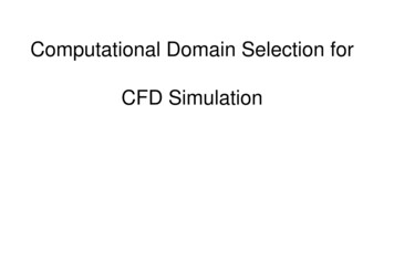
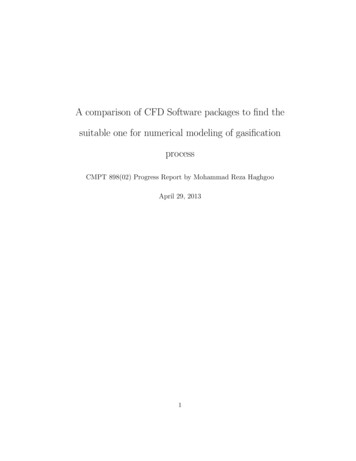
4.4Boundary ConditionsA uniform velocity is given at the inlet (left side). The pressure at the outlet(right side) is set to zero as the boundary condition assuming that the fluid isgoing out to the atmospheric pressure (zero relative). Zero gradient boundaryconditions have been applied on side walls.5Results (Laminar Flow)5.1Nek5000Figure 3 shows the velocity-magnitude field for Re 20 at final time. As weexpect, the result confirms that there is no vortex shedding at this Reynoldsnumber. However, two symmetric circulating region have been formed justbehind the cylinder.In Figure 4 the velocity-magnitude field for Re 100 at final time has beenrepresented. The Von Karman vortex street is clearly observable.5.2OpenFOAMFigure 5 depicts the velocity-magnitude field obtained by icoFoam solver inOpenFOAM for Re 100 at the final time.6ValidationIn analyzing a fluid flow over a cylinder, predicting the angle at which theboundary layer separates from the solid boundary is important. Here, wechoose this criterion to see how accurate the predicted results are.14
Figure 3: Velocity-magnitude field at Re 20, Nek5000Figure 4: Velocity-magnitude field at Re 100, Nek500015
Figure 5: Velocity-magnitude field at Re 100, OpenFOAMThe boundary layer separation occurs at the position on the cylinder wallwhere the shear stress is zero. Hence, at the separation point the normalgradient of velocity at the wall is zero i.e. If we draw the velocity profilenear the wall, the point at which the velocity is tangent to normal axis is theseparation point After which there is a rivers flow, as depicted in the Figure6. Figures 7, 8 and 9 show the velocity profile, obtained by OpenFOAM, ofFigure 6: Separation of the Boundary layer on the solid surface [15]16
the fluid near the cylinder wall at 90, 119 and 135 degree, respectively. Fromthe figures we can conclude that the separation occurs at about 119 degree.After that point the velocity near the wall will become negative and hence thefluid flows reversely.Figure 7: Velocity profile on the cylinder at 90 We plot the velocity profiles obtained by Nek5000 which predict the separation angle to approximately 118 degree.For the problem at hand some researchers measured the separation anglefor Re 100, experimentally [16]. They report it around 120 degree.Because the predicated results by OpenFOAM and Nek5000 are closeenough to experimental data we conclude that the procedure chosen for takingthe results is correct and accurate enough.17
Figure 8: Velocity profile on the cylinder at 119 Figure 9: Velocity profile on the cylinder at 135 18
7Turbulent FlowWe increase the Reynolds number to 600 at which the wakes formed in theflow become turbulent. We solve Reynolds Averaged Navier-Stokes Equations(RANS) using the k-ε modeling. U V 0 x y 2 U U P µ( U U x ) ρ u ρU ρV ρ t x y x x V V V P µ( V x ) ρ huviρ ρU ρV t x y y x(13)i µ( U) ρhuvi yh y(14)i2 µ( V) ρv yh y(15)It uses an eddy viscosity model (EVM) closure for the Reynolds stresstensor, hui uj i νt Ui Uj2 δij k xj xi3(16)This closure solves two additional transport equations for the turbulence kinetic energy, k and its dissipation rate, ε, which are then used to calculate thelocal eddy viscosityνt Cµk2ε(17)In which Cµ 0.09 .The turbulence kinetic energy is solved from a transport equation that is19
very similar to the generic transport equation: k k Uj t xj h νtσk ν k xji xj hui uj i Ui ε xj(18)Where σk 1The dissipation is solved from a very similar transport equation: ε ε Uj t xj h νtσε ν xj k xjiεε Cε1 P Cε2 εkk(19)Where σε 1.3, Cε1 1.44, Cε2 1.92This equation is tightly coupled to the k equation through the sourceterms.The near-wall treatment procedure, based on a straight extension of thewall functions, is included in solver.Numerical calculation schemes using turbulence models for the computation of turbulent flows usually adopt wall functions to bridge the viscoussublayer adjacent to a wall. This method of modeling the near-wall regionavoids the need to use numerous mesh points to resolve the very steep gradients prevailing in the viscous sublayer.With the wall-function approach the near-wall mesh point is placed in thefully turbulent fluid, and semi- analytical expressions called wall functions areemployed, which connect the wall conditions (e.g., wall shear stress and heatflux, wall temperature) to the dependent variables just outside the viscoussublayer.20
88.1Results (Turbulent)MfixMfix is mostly developed to address the gas-particle flows. Hence, almost allof the equations and turbulent models available in the Mfix is based on thefact that there is a two-phase flow being to be simulated. However, here wewant to visualize a single-phase flow over a cylinder. Although, it is hard butwe can do so by controlling the numerous parameters available in the software.Figure 10 Shows the velocity-magnitude field for Re 600 at the final time.Figure 10: Velocity-magnitude field at Re 600, Mfix21 page
ow it is necessary to develop a CFD software. The aim of this project is to make a comparison between CFD software packages in general and choose the a suitable one for modeling of gasi cation process. 1 Introduction Fast consumption of fossils fuels, energy security, and environme